Difference between revisions of "Projects:2016s2-246 Feral Cat Detector"
(→Approach) |
|||
| (20 intermediate revisions by the same user not shown) | |||
| Line 29: | Line 29: | ||
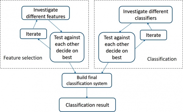
<div align="center">Figure 1 Project flow diagram </div> | <div align="center">Figure 1 Project flow diagram </div> | ||
| − | Based on the project of Richard & Yang in the last year, we build a alternative classification system which consist of two parts: feature selection and classification. In this project, instead of single feature, we have used feature combination which is proven could improve the classification performance. Moreover, we have test several classifiers to find which one is better and applied the better one in our system. | + | Based on the project of Richard & Yang in the last year [1][2], we build a alternative classification system which consist of two parts: feature selection and classification. In this project, instead of single feature, we have used feature combination which is proven could improve the classification performance. Moreover, we have test several classifiers to find which one is better and applied the better one in our system. |
In feature selection, we select 5 single features as base features: SIFT, PHOW, PHOG, LBP and SSIM. At first, we compare the performances of feature combination and single feature to find which way is better. Then, based on 5 base features to test all feature combinations and find the feature which can obtain the highest accuracy. | In feature selection, we select 5 single features as base features: SIFT, PHOW, PHOG, LBP and SSIM. At first, we compare the performances of feature combination and single feature to find which way is better. Then, based on 5 base features to test all feature combinations and find the feature which can obtain the highest accuracy. | ||
For the part of classifictoin, we verify the framework of AdaBoost can improve classifier’s performance firstly, and then find the best classifier among 4 classifiers, SVM, MKL-SVM, softmax, SVM+AdaBoost. | For the part of classifictoin, we verify the framework of AdaBoost can improve classifier’s performance firstly, and then find the best classifier among 4 classifiers, SVM, MKL-SVM, softmax, SVM+AdaBoost. | ||
| Line 41: | Line 41: | ||
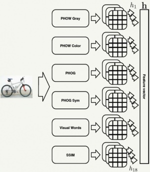
<div align="center">[[File:Feature extraction.jpg|300px]]</div> | <div align="center">[[File:Feature extraction.jpg|300px]]</div> | ||
| − | <div align="center">Figure 2 Feature extraction </div> | + | <div align="center">Figure 2 Feature extraction [3]</div> |
===Classification=== | ===Classification=== | ||
| Line 48: | Line 48: | ||
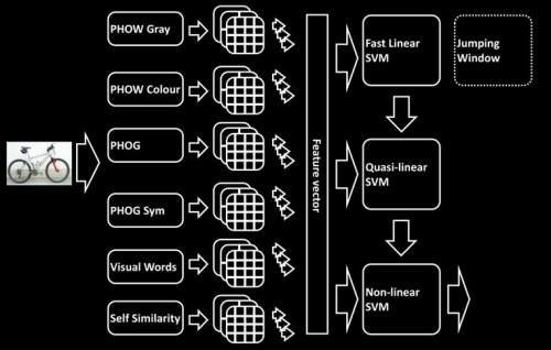
MKL-SVM is a cascaded SVM which is consisted of three internal SVM classifiers, i.e., fast linear SVM, quasi-linear SVM and non-linear SVM. Each classifier has its distinct kernel. The task of MKL-SVM is to compute kernel matrices of training and test images. Even though the histograms can represent the images, it still impossible to build a linear classifier for every class. Thus, we use a feature map in which the regions of interest (features) are linearly separable to help us find the optimal kernel. | MKL-SVM is a cascaded SVM which is consisted of three internal SVM classifiers, i.e., fast linear SVM, quasi-linear SVM and non-linear SVM. Each classifier has its distinct kernel. The task of MKL-SVM is to compute kernel matrices of training and test images. Even though the histograms can represent the images, it still impossible to build a linear classifier for every class. Thus, we use a feature map in which the regions of interest (features) are linearly separable to help us find the optimal kernel. | ||
<div align="center">[[File:Mkl-svm.jpg|500px]]</div> | <div align="center">[[File:Mkl-svm.jpg|500px]]</div> | ||
| − | <div align="center">Figure 3 Visual object detection via a MKL-SVM </div> | + | <div align="center">Figure 3 Visual object detection via a MKL-SVM [3]</div> |
| + | |||
| + | =='''Results analysis'''== | ||
| + | ===The classification accuracy improvement made by feature combination=== | ||
| + | |||
| + | <div align="center">[[File:Five features.jpg]]</div> | ||
| + | |||
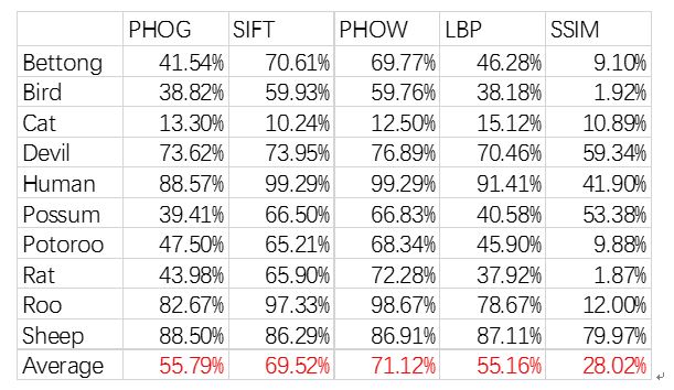
| + | <div align="center">Table 1 Classification accuracies of five features </div> | ||
| + | The classification results of this table all are average value by averaging three rounds’ results. Observing this table, we find SSIM feature has the worst performance whose average accuracy is 28.02%. PHOW is the most accurate one among these five features. Its average accuracy is 71.12%. For the other features, SIFT, PHOG and LBP, their average accuracies of 3 rounds are 69.52%, 55.79% and 55.16%, respectively. | ||
| + | |||
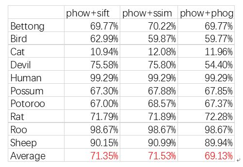
| + | Next stage, we will test performance of feature combination. The last step, we found that PHOW feature has the best performance. Thus, in this step, we combine it with other features, i.e., PHOW+SIFT, PHOW+SSIM, PHOW+PHOG. The following figure is the results of feature combination. | ||
| + | <div align="center">[[File:three combinations.jpg]]</div> | ||
| + | |||
| + | <div align="center">Table 2 Summarized results of three feature combinations </div> | ||
| + | Calculating the accuracies from the previous tables, we get the average accuracies of PHOW+SSIM, PHOW+SIFT, PHOW+PHOG, they are 71.53%, 71.35% and 69.13% separately. | ||
| + | Comparing above two tables, we know that the average accuracies of feature combination are higher than the accuracies of most single features. Even SSIM, the worst performance of single feature, also could obtain a satisfying result, 71.32%, after it being combined with PHOW. Hence, we conclude that the accuracy of classification system can get improvement after applying the method of feature combination. | ||
| + | |||
| + | ===The best performance feature combination in project=== | ||
| + | |||
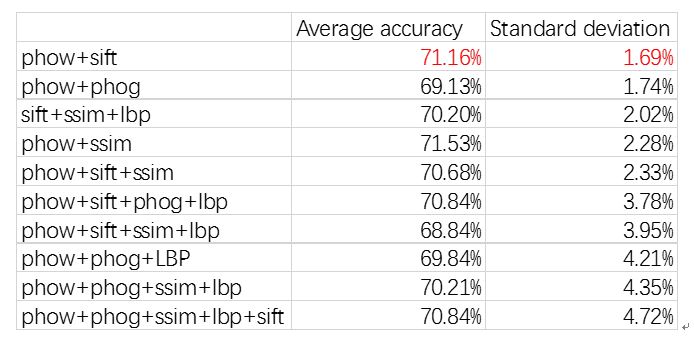
| + | The combination of PHOW and SIFT has a second highest accuracy, 71.16%, meanwhile, its standard deviation is the lowest. But, rest of feature combinations also are acceptable, their average accuracies approximately are 70% that lower a little bit than PHOW+SIFT’s. Especially, for PHOW+PHOG+SSIM+LBP+SIFT, it’s average accuracy is 70.84% and standard deviation is 4.72%, that means its has possibility to perform better than PHOW+SIFT in a certain test. Thus, we make a conclusion, the combining of PHOW and SIFT performances best for whole dataset, but the others are comparable. | ||
| + | <div align="center">[[File:top 10.jpg]]</div> | ||
| + | |||
| + | <div align="center">Table 3 Statistical data for best 10 feature combinations </div> | ||
| + | |||
| + | The combination of PHOW and SIFT has a second highest accuracy, 71.16%, meanwhile, its standard deviation is the lowest. But, rest of feature combinations also are acceptable, their average accuracies approximately are 70% that lower a little bit than PHOW+SIFT’s. Especially, for PHOW+PHOG+SSIM+LBP+SIFT, it’s average accuracy is 70.84% and standard deviation is 4.72%, that means its has possibility to perform better than PHOW+SIFT in a certain test. Thus, we make a conclusion, the combining of PHOW and SIFT performances best for whole dataset, but the others are comparable. | ||
| + | |||
| + | ===Practical results display=== | ||
| + | we build a confusion matrix of PHOW+SIFT to display its classification results in detail. Confusion matrix can visualize the system’s performance, the number of each column of confusion matrix represent the number of test images in a predicted category while the numbers of each row represent the number of test images in actual category. All correct predictions are located at the diagonal of matrix and marked red, the blue values are the total number of test images of each animal. | ||
| + | <div align="center">[[File:Phow+sift.jpg|600px]]</div> | ||
| + | |||
| + | <div align="center">Figure 4 Classification result of phow+sift </div> | ||
| + | Above figure shows one of classification results of PHOW+SIFT, we find the number of correct prediction of cat is 22 with 195 cat test images in total and most cat test images are classified as bird, human and sheep. | ||
| + | |||
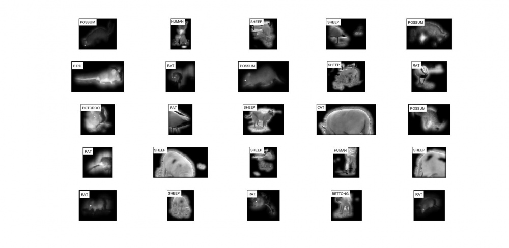
| + | Moreover, we show a practical classification result at below. There are 25 images with predicted class. | ||
| + | <div align="center">[[File:Wiki.jpg|1000px]]</div> | ||
| + | |||
| + | <div align="center">Figure 5 Practical classification results </div> | ||
| + | |||
| + | =='''Acknowledge'''== | ||
| + | For Dr Danny Gibbins & Dr Said Al-Sarawi, thanks for your guidance, advice and support. | ||
| + | |||
| + | For Richard Steenvoorde and Song Yang, thanks for your significantly important image dataset and effective system which inspires and helps us avoid hundreds of crooked roads. | ||
| + | |||
| + | =='''Reference'''== | ||
| + | [1]R. Steenvoorde, "Feral Cat Detector", master, The University of Adelaide, 2016. | ||
| + | |||
| + | [2]S. Yang, "Feral Cat Detector", master, The University of Adelaide, 2016. | ||
| + | |||
| + | [3]Vedaldi. Andrea, Varun. Gulshan, Manik. Varma, and Andrew. Zisserman, Multiple kernels for object detection, In Computer Vision, 2009 IEEE 12th International Conference on, pp. 606-613. IEEE, 2009. | ||
Latest revision as of 15:05, 5 June 2017
Introduction
Group members
Bolun Huang & Yan Chen
Supervisors
Dr. Danny Gibbins & Dr. Said Al-Sarawi
Background
In Australia, significant numbers of native wildlife are killed each year by feral cats and foxes. As part of their control and monitoring, field researchers and park managers are interested in low cost automated sensor systems that could be placed out in the field to detect the presence of feral cats and possibly even trigger control measures. The aim of this project is to examine a range of image and signal processing techniques that could be used to reliably detect the presence of a nearby feral cat or fox and distinguish it from other native animals such as wallabies and wombats. The possible range of sensors that might be used to achieve this include (but is not limited to) infra-red imaging cameras, ultrasonic detectors, and imaging range sensors (akin to say an x-box Kinect). Both the sensors and the processing unit (say a raspberry pi or A20 based mini board) would need to be low cost and potentially sometime in the future be able to operate in the field for days at a time. The two students would be required to develop both the processing techniques and a simple hardware implementation which demonstrates their solution.
Approach
Based on the project of Richard & Yang in the last year [1][2], we build a alternative classification system which consist of two parts: feature selection and classification. In this project, instead of single feature, we have used feature combination which is proven could improve the classification performance. Moreover, we have test several classifiers to find which one is better and applied the better one in our system. In feature selection, we select 5 single features as base features: SIFT, PHOW, PHOG, LBP and SSIM. At first, we compare the performances of feature combination and single feature to find which way is better. Then, based on 5 base features to test all feature combinations and find the feature which can obtain the highest accuracy. For the part of classifictoin, we verify the framework of AdaBoost can improve classifier’s performance firstly, and then find the best classifier among 4 classifiers, SVM, MKL-SVM, softmax, SVM+AdaBoost.
Technical details
Feature Selection
Suggestion from previous project:the more features we used to describe visual objects, the more accurate classification result we obtain.Thus we select 5 base features, SIFT, PHOG, PHOW, SSIM and LBP. These 5 features describe one image from different aspects. SIFT is a shape descriptor so that some attributes of visual entities cannot be obtained, such as texture, appearance and color. LBP has a satisfactory performance in detecting object’s texture. PHOW can provide us with more information about the position of image. PHOG is able to detect more features from different scale space. SSIM finds the same regions of interest from a lot of images, thus it can help system find the similar objects from different images.
After selecting base feature, we start to test the performances of single features. The first step is to randomly combine single features to create a feature combination Test all feature combinations. Next step i to combine features, we build the histograms of employed features, concatenate them into a larger histogram and convert this histogram into a vector by quantization.
Classification
We implement a new classifier--Multiple Kernel Learning SVM (MKL-SVM). It had been proven to be a useful tool for image classification and object recognition in a number of studies, where every image is represented by multiple sets of features and MKL-SVM is applied to combine different features sets. MKL-SVM is a cascaded SVM which is consisted of three internal SVM classifiers, i.e., fast linear SVM, quasi-linear SVM and non-linear SVM. Each classifier has its distinct kernel. The task of MKL-SVM is to compute kernel matrices of training and test images. Even though the histograms can represent the images, it still impossible to build a linear classifier for every class. Thus, we use a feature map in which the regions of interest (features) are linearly separable to help us find the optimal kernel.
Results analysis
The classification accuracy improvement made by feature combination
The classification results of this table all are average value by averaging three rounds’ results. Observing this table, we find SSIM feature has the worst performance whose average accuracy is 28.02%. PHOW is the most accurate one among these five features. Its average accuracy is 71.12%. For the other features, SIFT, PHOG and LBP, their average accuracies of 3 rounds are 69.52%, 55.79% and 55.16%, respectively.
Next stage, we will test performance of feature combination. The last step, we found that PHOW feature has the best performance. Thus, in this step, we combine it with other features, i.e., PHOW+SIFT, PHOW+SSIM, PHOW+PHOG. The following figure is the results of feature combination.
Calculating the accuracies from the previous tables, we get the average accuracies of PHOW+SSIM, PHOW+SIFT, PHOW+PHOG, they are 71.53%, 71.35% and 69.13% separately. Comparing above two tables, we know that the average accuracies of feature combination are higher than the accuracies of most single features. Even SSIM, the worst performance of single feature, also could obtain a satisfying result, 71.32%, after it being combined with PHOW. Hence, we conclude that the accuracy of classification system can get improvement after applying the method of feature combination.
The best performance feature combination in project
The combination of PHOW and SIFT has a second highest accuracy, 71.16%, meanwhile, its standard deviation is the lowest. But, rest of feature combinations also are acceptable, their average accuracies approximately are 70% that lower a little bit than PHOW+SIFT’s. Especially, for PHOW+PHOG+SSIM+LBP+SIFT, it’s average accuracy is 70.84% and standard deviation is 4.72%, that means its has possibility to perform better than PHOW+SIFT in a certain test. Thus, we make a conclusion, the combining of PHOW and SIFT performances best for whole dataset, but the others are comparable.
The combination of PHOW and SIFT has a second highest accuracy, 71.16%, meanwhile, its standard deviation is the lowest. But, rest of feature combinations also are acceptable, their average accuracies approximately are 70% that lower a little bit than PHOW+SIFT’s. Especially, for PHOW+PHOG+SSIM+LBP+SIFT, it’s average accuracy is 70.84% and standard deviation is 4.72%, that means its has possibility to perform better than PHOW+SIFT in a certain test. Thus, we make a conclusion, the combining of PHOW and SIFT performances best for whole dataset, but the others are comparable.
Practical results display
we build a confusion matrix of PHOW+SIFT to display its classification results in detail. Confusion matrix can visualize the system’s performance, the number of each column of confusion matrix represent the number of test images in a predicted category while the numbers of each row represent the number of test images in actual category. All correct predictions are located at the diagonal of matrix and marked red, the blue values are the total number of test images of each animal.
Above figure shows one of classification results of PHOW+SIFT, we find the number of correct prediction of cat is 22 with 195 cat test images in total and most cat test images are classified as bird, human and sheep.
Moreover, we show a practical classification result at below. There are 25 images with predicted class.
Acknowledge
For Dr Danny Gibbins & Dr Said Al-Sarawi, thanks for your guidance, advice and support.
For Richard Steenvoorde and Song Yang, thanks for your significantly important image dataset and effective system which inspires and helps us avoid hundreds of crooked roads.
Reference
[1]R. Steenvoorde, "Feral Cat Detector", master, The University of Adelaide, 2016.
[2]S. Yang, "Feral Cat Detector", master, The University of Adelaide, 2016.
[3]Vedaldi. Andrea, Varun. Gulshan, Manik. Varma, and Andrew. Zisserman, Multiple kernels for object detection, In Computer Vision, 2009 IEEE 12th International Conference on, pp. 606-613. IEEE, 2009.
