Difference between revisions of "Projects:2014s2-80 Swinging Crane Project"
(→Fuzzification design) |
(→Fuzzification design) |
||
| Line 108: | Line 108: | ||
==== Fuzzification design ==== | ==== Fuzzification design ==== | ||
The fuzzyfication process uses fuzzy state variables to describe the system. Assume the state variables and control variable are: | The fuzzyfication process uses fuzzy state variables to describe the system. Assume the state variables and control variable are: | ||
| − | [[File: | + | [[File:Fuzzyfication_errors.png]] |
The state variables considered can be positive, zero or negative, also can be large and small. Presume there are 5 quantified intervals set for input variables, in which are “negative large” (NL), “negative small” (NS), “zero” (ZR), “positive small” (PS) and “positive large” (PL). While there are 5 quantified regions set for output, in which are “large acceleration” (LA), “slight acceleration” (SA), “zero acceleration” (ZA), “slight braking” (SB) and “large braking” (LB). | The state variables considered can be positive, zero or negative, also can be large and small. Presume there are 5 quantified intervals set for input variables, in which are “negative large” (NL), “negative small” (NS), “zero” (ZR), “positive small” (PS) and “positive large” (PL). While there are 5 quantified regions set for output, in which are “large acceleration” (LA), “slight acceleration” (SA), “zero acceleration” (ZA), “slight braking” (SB) and “large braking” (LB). | ||
Revision as of 22:28, 6 May 2015
Project aim: Swinging Crane project is aim to transporting a payload from one place to another and reducing the consuming time as much as possible.
Contents
Project introduction
Technical background
Gantry cranes are wildly used in industry, for lifting heavy objects by a hoist which is fitted in a hoist trolley and can move horizontally on a rail or pair of rails fitted under a beam.
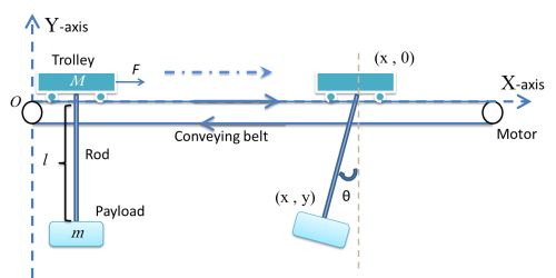
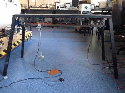
Figure 1 demonstrates the model of swinging crane, the DC motor controls the trolley to horizontally move a load in a short distance. There are two encoders to record the data, one is the moving distance, and another is sway angle of the load. By giving a signal from operation control system, it will generate a DC current from a current source, then injecting it into a motor, which would drive the conveyor belt. There is a trolley placed on one side of the belt, and start moving towards another side. At the bottom of the trolley, using a rod stand for the hoist, connect with a load. At the start of transporting the loads, it will cause accelerated, corresponds to a traction force, effect on the trolley. There occur an angle between the rod and vertical. After the trolley stops, the loads may turn to oscillate. If the initial angle large, the oscillation duration roses, which is a potential risk to the people on the ground.
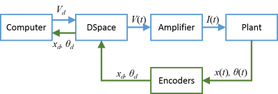
The system is operated inside a flow, shown as Figure 2. Input signal is generated from Simulink, goes into the plant through dSPACE and amplifier. The outputs of the plant are measured by two encoders, and send back to dSPACE, finally transfer to the computer. The dSPACE and amplifier components will introduce later. The plant is the real model of the system, the transfer relationship is shown in Figure 3. The current flows into DC motor, which drives the belt on the grid. The trolley is bind on the belt, thus it has the same acceleration with the belt. There are two outputs from the, the trolley position and the swinging angle of the pendulum.
Motivation
The gantry crane system could be identified into separate sections: linear motion and swinging pendulum. The goal is to minimum the time used to transport loads and reduce the swinging oscillation as minimize as possible. The pendulum was studied by Galileo, Huygens, Newton, Hooke and all the leading figures of 17th-century science. Since the long history on the study, pendulum theory has been almost perfect, but still exist imperfection in applied to practical. In this project, the basic model is simple gravity pendulum. To analyse the motion parameters of pendulum, Newton’s classical mechanics Laws are applied. In traditional education, Newton’s lows are taught in high-school physics lecture. The theorem is abstract to student, and divorced from the practical application. The gantry crane system is a representative application, and easy to understand, thus it is suitable for demonstration teaching purpose.
Objectives
The aim of swinging crane project is to demonstrate research component of project, examine and improve last year’s project, perform analysis, show understanding of theoretical principles, simulations and experiments, then improve system robustness, calculating instantaneous energy and optimize system motion trajectories. The 5 objectives of this project are shown as bellow:
1.Modelling of system – physical principles, approximates which can be used to simplify model (e.g. linearized model).
2.Selection of reference trajectories-trade-offs, constraints, optimization.
3.Calculation and control of “energy” stored in pendulum-means for damping energy.
4.Simulation of system- investigates and checks performance.
5.Experimental demonstration- interfacing operation, model verification.
Background
Previous work
The swinging crane real system is designed by the workshop of University of Adelaide. Some analysis has been done by previous group, a simple PID control and current manual control have also been developed. Thus some data of the model could use by directly looking up their reports.
Figure 4 gantry crane system is studied by last year project group. This model is based on lumped-mass model, which ignore the mass and the elongation of the rod caused by the tension force. Both of the trolley and payload are considered as point mass and moving in two-dimensional x-y plane.
System modelling
Simple pendulum model
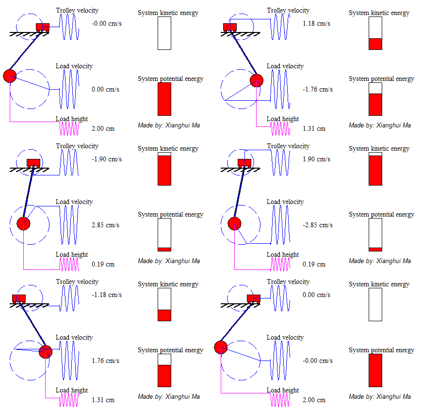
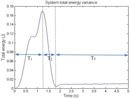
System total energy is the summation of kinetic energy of the trolley, the potential energy and kinetic energy of pendulum load. The animation on the left shows a free-trolley-position movement demonstration without friction or air-drag. Consider a trail of total energy in a system process, shows as Figure 5, in where T1 is the acceleration time period, T2 is the deceleration period and T3 is the remain oscillation period. The magnitude of system total energy in T3 is a constant value with frictionless assumption. The left animation illustrates the system remaining oscillation relationship in T3.
System equations
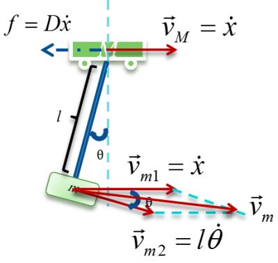
According to Figure 6, the system total energy could be expressed as:
Taking the force relation, the system transfer function is
 ,
if the pendulum swing a small angle(i.e.less than 10 degrees), the above equations could be reduced to
 .
.
By taking the Laplace transform, the system transfer function is
![]() .
.
The above equations could also write as state-space model form. Assume the state variable ![]() , and state equation
, and state equation ![]() the state matrices are
the state matrices are  ,
, and
and .
.
Control methods designing
PID control
Fuzzy-logic control
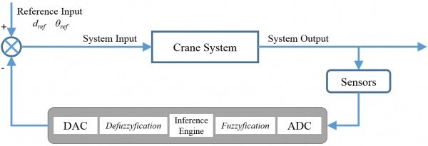
Fuzzy logic control is a rule-based control method. The controller is designed with a set of fuzzy rules for both input and output sides. Figure 10 shows the basic structure of a fuzzy control system.
In classic control field, the precision of a control system modelling effects the system behaviour most. The dynamic information of the system state could help achieve the goal of accuracy control. However, the number of the state variables are too much for a complex system, and they may have influence to each other, thus it is difficult to describe the system state correctly. Fuzzy logic control uses the idea and theory of fuzzy algorithms to describe the system state. Fuzzy control is a nonlinear control method, and it also belongs to intelligent control branch. In general, a control engineer will use classic algorithms (of the classic PD type, for example) if the system can be modelled and fuzzy algorithms (of the fuzzy PD type, for example) if the system cannot be modeled (or can only be partly modeled).
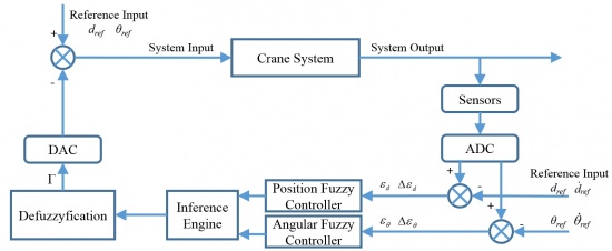
In this project, there are 4 state variables, which defined in previous. Based these variables, two fuzzy controllers are used. The system simulation diagram shows as Figure 11.
Fuzzification design
The fuzzyfication process uses fuzzy state variables to describe the system. Assume the state variables and control variable are: File:Fuzzyfication errors.png
The state variables considered can be positive, zero or negative, also can be large and small. Presume there are 5 quantified intervals set for input variables, in which are “negative large” (NL), “negative small” (NS), “zero” (ZR), “positive small” (PS) and “positive large” (PL). While there are 5 quantified regions set for output, in which are “large acceleration” (LA), “slight acceleration” (SA), “zero acceleration” (ZA), “slight braking” (SB) and “large braking” (LB).
Position manual control
Hardware test and interfacing
Results comparison
Conclusion
Group members
Liyan Yi
Xianghui Ma
Supervisors
Dr.Wen Soong [1]
Dr Braden Phillips [2]
