Projects:2018s1-181 BMW Autonomous Vehicle
Contents
Students
Corey Miller
Kaifeng Ren
Muhammad Sufyaan Bin Mohd Faiz
Ovini Amaya Perera
Yiduo Yin
Supervisors
Associate Professor Nesimi Ertugral
Mr. Robert Dollinger
Project Description
Software Development
This projects main focus is on MPC development for a steering system of the BMW autonomous vehicle. During this project, Model Predictive Controller toolbox in MATLAB Simulink will be used to develop the MPC controller which suits in our project. In addition, the vehicle model which was provided by Robert Dollinger in 2016 could not be used in Model Predictive Controller Toolbox in MATLAB due to errors. Therefore, In the software part, a new vehicle model will be developed and a Model Predictive Controller will be developed and used in the simulation part of this project. New software call Driving Scenario Designer will also be used to develop the reference track for simulating the new vehicle model and controller.
MPC Introduction
Stability and safety are the most important factors of autonomous driving. MPC is a controller which has 2 important advantages to achieve the stability and safety of the autonomous vehicle’s steering system.
■ Advantage1: Constraints Handling There are a lot of constraints (physical limitations) which need to be overcome when the car is driving on the road. MPC can handle constraints systematically and produce feasible solutions for our car. Its ability of constraints handling can provide stability and safety for our autonomous vehicle.
■ Advantage2: Optimization of the result Although the result returned by MPC may not match the reference trajectory precisely, the result can still be optimized as hard as possible to get close to the given trajectory.
Vehicle Model
The vehicle model used for the system will be summarized using state space representation: modelling the physical vehicle as a set of input, output and state variables (variables that change over time depending on the input variables at a specific instance). The benefits that state space representation has over other modelling techniques is that it allows input data from multiple sources to be used simultaneously in the same model to estimate a single dynamic vehicle parameter and provides a convenient way to analyses multiple inputs and outputs. Comparing this to the frequency domain, state-space representation is not limited to systems with linear components and zero initial conditions and is more efficient than having to write input × output number of Laplace transforms to describe the system.
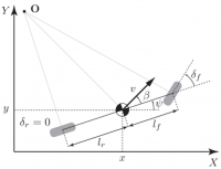
To model the vehicle in state space representation, a linear single-track model (also known as the bicycle model) was used to describe the lateral dynamics of the vehicle. The bicycle model simplifies the dynamics of a vehicle by taking the front and rear axles and treating them as singular wheels. This simplifies the lateral dynamics of the vehicle by reducing the degrees of freedom from having 4 wheels to 2 wheels, hence fewer equations are required to describe the vehicle model.
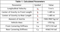
The state vector used in the vehicle model consisted of the vehicle slip angle (β), yaw (ψ), yaw rate and the lateral position (y). This allowed for the calculations of the vehicles longitudinal and lateral positions and yaw at each timestep with respect to a steering angle input (𝛿).The parameters for the state space model can be seen in the calculated parameters table.
The developed simulink vehicle model based off this state space model can be broken into 3 seperate sections. Section 1 takes all the relevant parameters from the matlab script file and loads them into the model to be used. Section 2 calculates the state vector and Section 3 uses the parameters inside the state vector to calculate the longitudinal and lateral position of the vehicle.
Model Predictive Controller
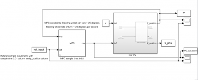
The model predictive controller subsystem takes the lateral position of the vehicle model as an input and compares it against the reference path's lateral position of where the vehicle be. Based off the deviation from where the vehicle is and where it should be, the MPC adjusts the steering wheel angle of the vehicle, turning the wheels to head the vehicle to follow the reference path. What makes model predictive control able to control a vehicle to follow reference path more accurately than other control strategies is its ability to "predict the future". During each timestep (in this projects case 20ms) the lateral position deviation problem is optimized over finite set of timesteps. This is known as the prediction horizon - how far the MPC sees into the future. For each of these future timesteps, the MPC calculates the required steering angle to optimize the deviation problem. The MPC then only executes finite range of these timestep steering angle commands. This is known as the control horizon - how long the MPC executes 1 optimization problem. The reason a control horizon does not execute all the prediction horizon estimated steering angles is that a contingency may occur (such as an object entering the vehicles path) that the optimization problem did not account for. Therefore at each timestep, a new optimization problem is solved with only the first few steps being sent to the steering wheel.
When designing the MPC submodule in MPC toolbox in MATLAB, a prediction horizon of 20 samples (0.4 seconds into the future) was used as it provided the MPC a clear understanding of the path ahead while maintaining fast processing speed. A control horizon of 1 sample was used as the performance of the module was not improved from increasing the control horizon. For passenger comfort, constraints were set on the steering angle output of the MPC that was being sent to the vehicle. This constraints included reducing how far the steering angle could turn from -25 degrees to +25 degrees, allowing for wide turns. The rate of how quickly the steering wheel turn was also constrained to 25 degrees per second, allowing for a smooth transition into a turn without the steering wheel rapidly changing the direction of the vehicle.
The diagram belows shows the fully connected MPC system with an input longitudinal velocity and reference path (consisting of a lateral position at each timestep) and outputting the lateral position and steering angle of the vehicle.
Simulation Results
To test the performance of the MPC and vehicle model, the system was placed into 3 different scenarios that simulated real world traffic conditions. These scenarios were designed using Driving Scenario Designer MATLAB Application. Simulation 1 involved the vehicle performing a lane change maneuver in a double-laned road.
Software Part Future Work
The MPC controller that we developed can only acquire good performance results when the speed is 18km/h. In some cases, there will be 1.5 meters oversteer on the Y position when the vehicle tries to track and approach the reference path at the beginning. Therefore, we thought this oversteer was caused by the set parameters which were not properly measured. These parameters include cornering stiffness and moment of inertia of the vehicle. Hence, as a further development, a parameter estimator may be required and developed.
Secondly, as I mentioned above that the vehicle can only perform well at 18km/h, so an adaptive MPC controller may be needed to allow the vehicle to follow the reference path at different speeds.
By using the vehicle model, we observed that when the vehicle's velocity get close to 0, the state space model becomes unstable which is another problem that needs to be solved in the future work.
Hardware Part
...due Sunday night.


