Projects:2016s1-120 Attacking Cancer with Signal Processing

---

Project Information

Topic: Attacking Cancer with Signal Processing

Supervisors：Dr. Andrew Allison

Adviser: Prof. Derek Abbott

Project members: Jin Hu Mohammed Said Al-Wahaibi

Introduction

Cancer is one of the most devastating unsolved medical problems. Only 7% of cancer patients on average have a hope of recovery. New approach to solve the problem is to fight the cancer by strengthening the human body's own immune system, by improving the timing of treatment, using signal processing. CRP is produced by the liver and adipocytes in response to inflammation. People who infected by cancer have a different CRP level comparing to healthy ones. Study showed that the best time to apply the immune therapy is when the CRP level is low.

Motivation and Objectives

The main focus of the project is to improve the existing treatment, by improving the timing. The project uses signal processing to estimate the optimal treatment time. The ultimate goal is that this project will help extending human lives.

Previous Studies

In 2009,Dr. Brendon Coventry and his colleagues used Low-Reactive Protein (L-CRP) test to obtain high sensitivity data of CRP. And they found the CRP levels are periodic with the cycle of 7 days.

In 2014, Dr. Mutsa Madondo and his colleagues did their research ,they used Enzyme-Linked ImmunoSorbent Assay(ELISA) to obtain blood samples from patients at seven different times in 12 days' period.Then they claimed that CRP levels and Treg and Teff frequencies did not appear to be oscillatory.

Background

The CRP level of a cancer patients is differing from a healthy human. As the CRP response to inflammations, the change in it level might be periodic and accrue in cycles. The CRP data we have a noisy and irregularly sampled. To separate the noise from the signal we use Fast Fourier Transform techniques and Lomb Periodogram. Both methods are valid way to separate the noise from the signal. We use both method to make sure of getting a valid signal and reducing the possibility of false positives.

Noise Floor

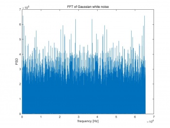
The noise floor is the Fourier transform of noise and unwanted signal. Figure 1 shows the FFT result of Gaussian white noise, which is very noisy and no pure peak can be found. If performing FFT on a noiseless signal , a pure peak will appear on the power spectral density (PSD). For noisy signal, even the peak can be obtained on PSD, the FFT of noise still shows in the background.

Figure 1. Noise Floor

Kolmogorov–Smirnov Test

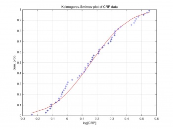
Kolmogorov–Smirnov test can compare a sample with a reference probability distribution. Figure 2 shows the Kolmogorov–Smirnov test of the raw CRP data. The CRP data are formed in log scale，and follow the Gaussian distribution. Therefore, we can generate Gaussian random pseudo-data by creating Gaussian random variables based on the log scale CRP data. pseudo_data=(random×σ)+μ

Figure 2. Kolmogorov–Smirnov Test of CRP Data

De-trending CRP Data

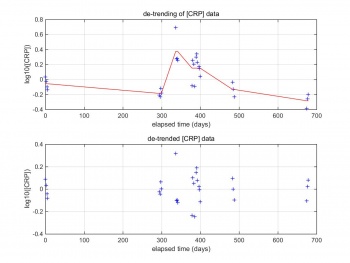
By taking out the trend from our CRP data, it enables us to focus our analysis on the fluctuations in the data. A linear trend typically indicates a systematic increase or decrease in the data, which gives a method for analyzing shorter-term cyclical patterns. These patterns can then be used to more effectively identify major turning points in the longer-term cycle which is what this project is aiming for.as mentioned before the data being treated as separate monitoring period (MP) if the measurement been taken seven days apart. Figure 3 shows the CRP reading for patient No.10. The red line of the top one is the DC component which that go in the middle of each monitoring period. So by taking the DC component will help us identify cyclical patterns. The bottom image is CRP data after removing the DC component.

Figure 3. De-trend of Patient No.10 CRP Data

Analysing the CRP Data

Power Spectral Density

There are two methods to estimate the Power Spectral Density (PSD), one applies fast Fourier transform (FFT) of the re-sampled CRP data, another is using Least-squares spectral analysis (LSSA) of the raw CRP data.

Fast Fourier Transform

The technical challenging of this project is the available CRP data is irregular. When using Matlab to apply FFT of a signal, the samples should be uniform space. So the raw data needs to be interpolated values by spline method, Kriging interpolation or basis function.Spline method can fit the raw data well, but the overshoots is a big issue that may cause the FFT result distorted. In terms of Kriging interpolation, it is too complex to complete the interpolation processing.Even the basis function does not fit the raw data as well as the spline method,the result of basis function is feasible. Moreover, basis function can remove the overshoot which reduces it to the mean level of log scale CRP data. So we Gaussian basis function is the best choose for re-sampling.

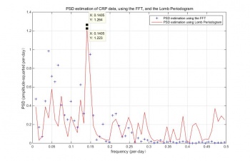
FFT is a useful analytical tool applied in diverse fields, as an effective computational method to calculate a Fourier transform. When analyzing a signal, FFT decreases the number of calculations in order to quickly generate a Fourier transform. So, the properties of FFT and noise processes is well understood. Moreover, FFT and Rayleigh Energy Theorem can use for checking the normalization of calculations. In Figure 4, the blue points are the PSD estimation results of performing FFT. There is an observable peak located at the frequency of 0.1405 per day and the periodic of the peak is 7.117 days.

Lomb Periodogram

LSSA is also called Lomb periodogram, which can apply for irregular samples without re-sampling the data or invent other values . The red line in Figure 4 is the PSD estimation results using Lomb periodogram. The peak locates at the frequency of 0.1405 per day and the periodic of the peak is 7.117 days.

Even though there are some differences between the two results in vision, the peak frequencies of FFT and Lomb periodogram are similar. Both the peak frequencies locate at 0.1405 per day and the periodic at peaks are close to 7 days. So, these two methods are feasible for estimating PSD of log scale CRP data. However, some CRP values are estimated when performing FFT. The data used in Lomb periodogram are all measured value. So,Lomb Periodogram have more details data comparing to FFT as there might some data lost in the re-sampling process before using the FFT.

Figure 4. PSD Estimation Using FFT and Lomb Periodogram

Sine Wave Fitting

The equation of fitting cure is: y_i=Acos(ωt_i )+Bsin(ωt_i )+C

The coefficient A, coefficient B , constant offset C ,ω and initial parameters are the unknown value will be obtained by using the least square method. The frequency of peak will be used to create the initial parameters. According to the fundamental theorem of algebra, each monitoring periodic should contain at least 5 data for sine-wave fitting.

Based on the periodicity of the sine curve, we can predict the time of the next minimum by using the last fitted data.

The minimum is at ωt_i+θ=2Nπ-2π

To estimate the next minimum time, N= ceil((ωt_Last+θ+π/2)/2π) The next minimum time: t_min=(N∙2π-π/2-θ)/ω