Projects:2017s1-101 Classifying Network Traffic Flows with Deep-Learning

Project Team

Clinton Page

Daniel Smit

Kyle Millar

Supervisors

Dr Cheng-Chew Lim

Dr Hong-Gunn Chew

Dr Adriel Cheng (DST Group)

Introduction

The internet has become a key facilitator of large-scale global communications and is vital in providing an immeasurable number of services every day. With the ever-expanding growth of internet use, it is critical to effectively manage the underlying networks that hold it together. Network traffic classification plays a crucial role in this management, providing quality of service, forecasting future trends, and detecting potential security threats. For these reasons, accurate network traffic classification is of great interest to internet service providers (ISPs), large-scale enterprise companies, and government agencies alike.

Current methods of network traffic classification have become less effective in recent years due to the increasing trend of obscuring network activity, whether it be for security, priority, or malicious intent [1, 2, 3]. Therefore, in today’s network there arises a need for a more effective classification algorithm to handle these conditions.

Within this research, the following types of classifiers were produced using three different methods:

• Application traffic classification – in which the flows of 10 common web-based protocols or applications were classified as their respective classes, and unknown or other flows were classified as Other.
• Malicious classification – in which the flows of 6 malicious traffic types were classified as their respective classes, and non-malicious application or other flows were classified as Other.
• Malicious detection, in which the model would output whether or not the traffic was malicious. This model used two classes – malicious and non-malicious.

Objectives

• Gain knowledge about the application of deep-learning for classifying network traffic flows

• Conduct experiments on synthetic traffic flows and/or make use of communications flow data from real-life enterprise networks

• Develop network traffic classifying software using deep-learning techniques to an acceptable accuracy when comparing against the results of previous years

Relevant Work

Extensive research has been performed on network traffic classification. Common techniques include port-based classification and deep pack inspection (DPI). Port-based classification performs poorly due to the usage of non-standard port numbers, and DPI requires updates to recognise unseen classes of network traffic. Moore and Papagiannaki [4] found that using port-based classification as the sole classifier resulted in classification accuracies of less than 70%. nDPI, an open-source tool for investigating traffic using DPI, shows that a high classification accuracy (around 99%) can be achieved for standard applications but will deteriorate depending on how common the application is or whether it has been encrypted [5].

The use of machine learning techniques for network traffic classification has therefore been researched extensively to tackle the problems with these traditional methods. Previous iterations of this project have investigated using various machine learning techniques to preform network classification. In the 2014, tree based and support vector machines (SVM) algorithms were investigated. Using the Universitat Polit`ecnica de Catalunya (UPC) data set [6] they were able to classify botnet traffic from legitimate traffic with up to 94% classification accuracy using decision trees and 89% classification accuracy using SVM techniques [7]. In 2016, 10 graph-based methods which utilised spatial traffic statistics were explored and achieved classification accuracies up to 95% using the same UPC data set [8].

Auld et al. [3] investigated the use of statistical data (e.g., number of packets per flow) as inputs to a neural network. The study used Bayesian Neural Networks and created a model using 246 selected flow level features. A list of the most valuable features was then created based on the weightings in the neural network, and included in the report. With this method, an accuracy of 95.8% was achieved with over 200 features.

Trivedi et al. [9] found similar results utilising a neural network to classify network traffic based upon the variance of packet lengths. Comparing the neural network against a clustering approach, it was found that a neural network could both achieve a better classification as well as take less time to train.

As the utilisation of deep learning has been a relatively recent addition to the field of machine learning, only few papers have considered their use in network traffic classification. Wang [1] showed that utilising the first one thousand bytes of a network flow’s payload could prove an effective input for a deep (multilayered) neural network. Although the paper was lacking in overall detail about their implementation and information about the data set used, the results showed promising results for the utilisation of deep learning in network traffic classification.

Background

Network Flows

The term ‘flow’ can be thought of as conversation between two end points on a network. These two end points will exchange packets with each other until this conversation ends. Packets consists of two sections, the header section which holds information about the packet (e.g., destination and source address), and the payload section which holds the message that will be delivered to the recipient. An individual flow has been defined as the unidirectional or bidirectional exchange of packets containing the same five key properties [10]:

• Destination IP address
• Source IP address
• Destination port address
• Source port address
• Transport layer protocol (TCP or UDP).

Machine Learning and Deep Learning

ML is a subset of artificial intelligence (AI) that uses pattern recognition to classify or make predictions from a given set of data. This project will focus on one area of ML in particular, supervised learning. Supervised learning is a type of learning algorithm which uses the desired output (in the case of this report, the correct classification of network traffic) to assess the performance of a model and make corrections based upon the difference between its prediction and the correct classification [11].

Artificial neural networks (ANN, or alternatively simplified to NN) are a subset of machine learning that are formed on the basis of designing mathematical models to mimic how biological neural networks compute information. There are many different types of NNs but the foundation of which, is a network of simple processors, referred to as nodes or neurons, which communicate through numerous connections to other nodes within the network [12] (refer to Figure 2). NN are structured in layers; it is these layers that hold the distinction between deep neural networks and other NNs. A typical NN will be divided into three layers, the input, hidden, and output layer. When a NN is made up of multiple hidden layers it is said to be a Deep Neural Network (DNN). Deep learning is the process of using these deep neural networks for machine learning.

Convolutional Neural Networks (CNNs) are a type of NN that differ from traditional feed-forward reverse propagation by how data is presented to the network. CNNs are passed in data in the form of an image which is then filtered and processed by a neural network to extract an output prediction. Convolutional neural networks have been shown in industry to achieve high performance but require their input to be in the form of an image.

Precision and Recall

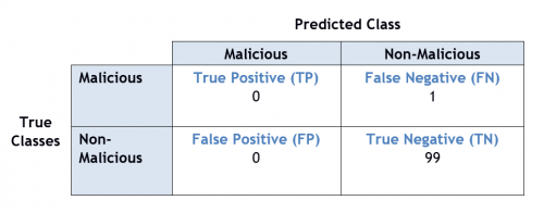
In terms of comparing ML algorithms it is not always prudent to compare the overall accuracy of the models. Take for example a ML model which aims to identify all malicious sample in a set of 100 results. If there is only 1 malicious sample in this set, the model can still achieve a 99% accuracy by classifying every sample as non-malicious. Two metrics that help to measure this imbalance are precision and recall [13].

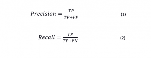
Precision is defined as the number of times a class is correctly identified over the number of times that the class was predicted. This is useful when assessing how reliable a prediction can be made. Recall is defined as how many times a class is correctly identified over the total number of that class within the data set. This shows how well a class can be identified against the other classes. [19].

A confusion matrix is used to show the prediction versus the true classification for every class in the system. For example, a confusion matrix for the previous example can be seen below. It should be noted that here the positive class has been identified as the malicious sample. It can be seen that as the example model does not correctly identify any malignant samples it will have a precision and recall of zero.

Method

An overview of each approach to classification

One of the major questions faced in this project was how network traffic should be represented to a deep neural network. To address this challenge, the research was divided into three main phases, each proposing a new input strategy.

• Phase 1: Drawing from research conducted by Wang [1], Phase 1 explored using patterns found in the payload sections to preform flow classification. In its essence, this is the same method used by deep packet inspection, a widely used method of traffic classification. However, by utilising deep learning to find these patterns it is no longer limited to just those that can be detected by humans.
• Phase 2: Assessed the viability of using statistical features derived from a flow as inputs to a deep neural network. As these features have a higher tolerance to encryption methods and are harder to obscure, this phase aimed to construct a more robust classifier. There have been many studies utilising this method in machine learning, the aim of this phase was extending this research by utilising a deep learning classifier.
• Phase 3: By exploiting classification methods typically found in image recognition, Phase 3 focused on representing network traffic as images based on the network traffic data and then using a convolutional neural network for classification.

A method of calculating the confidence of a prediction was also implemented and for each classification type and is shown in the results section for each phase.

This research aims to provide an extensive analysis of deep learning’s performance on traffic classification using a multitude of neural network configurations. In machine learning the parameters selected before a classifier trains are called the hyperparameters. This is to avoid confusion with the self-defined parameters the classifier will set through training. Six model hyperparameters were investigated to determine their effect on network traffic classification and are described below. TensorFlow [14] was then utilised to build and evaluate the different model architectures.

Hyperparameters	Description and Significance
Number of nodes in the hidden layer(s)	Increases the model’s degrees of freedom, as the number of processing units and connections is increased.
Number of hidden layers	Each layer generates a higher order representation of the input data.
Padding style	Padding a flow with either zeros or random values such that each flow meets the required input length.
Input length	The number of bytes used from each bi-directional flow. As each input byte maps to a respective node in the input layer, the number of bytes used also determines how many nodes are present in the input layer.
Training/Optimization algorithm	Responsible for adjusting the connection weights to minimize the cost function.
Activation functions	Responsible for detecting non-linear patterns in the input data.
Category encoding	How the inputs and outputs are encoded.

Data set

Deep learning benefits from a large and extensive data set and as supervised learning was to be used, this data set must also be labelled. Due to these reasons, the UNSW-NB15 data set [3, 21] was chosen as the basis for this research. Released in 2015, UNSW-NB15 contains a capture of around 1 million bi-directional flows, made up of both application and malicious traffic. This data set was generated over two separate days, for approximately 15 hours on each of the days. The data set was provided in two distinct sets of packet captures from the 22 nd of January 2015 and 17 th of February 2015. To ensure that the developed model generalises well with new data, the proposed use of this data set for this phase was to train using one set, and test with the other. By using the different sets recorded at different times, our classification results may correspond more closely to the results of classification when applied in a real scenario.

From this data set, a selection of application and malicious classes was chosen. For the application classes, the ten largest represented applications were selected. The remaining flows were group into an 11th “Unknown” class. Two different versions of data sets were then made: one for general application network traffic classification, and another for malicious traffic classification. These were developed to provide an approximately equal number of classes for training.

For the application data set, the data set from 22 Jan 2015 was used for training, while the 17 Feb 2015 data set was split into testing and validation sets, with proportions of 60% and 40%. This resulted in overall proportions of 50% training, 30% testing and 20% validation. The malicious data sets were created by merging both the 22 Jan 2015 and 17 Feb 2015 data sets together, and creating a data set of evenly distributed malicious classes, as well as an equal sized general application class. While the training set is made from the 22 Jan 2015 data set, the testing and validation sets were made by randomly sorting the 17 Feb 2015 data set and splitting the results into the 60%/40% distribution. Additionally, due to the small number of instances of the four smallest malicious classes: ANALYSIS, BACKDOOR, SHELLCODE and WORMS, these were grouped together into a single class called OTHER_MALICIOUS.

Application Protocols	Malicious Classes
DNS	Exploits
FTP	Fuzzers
FTP-DATA	Generic
Mail (POP3, SMTP, IMAP)	DOS
SSH	Reconnaissance
P2P (eDonkey, Bittorrent)	Other Malicious
NFS
HTTP
BGP
OSCAR
Unknown

Phase 1

An overview of how data was represented in Phase 1

Phase 1 explored network classification based on the first one thousand bytes in the payload of a bi-directional flow. As a flow is made of multiple packets, each containing their own payload, these payload sections were concatenated together until the required number of bytes was met. The data was then used to train a feedforward-backpropagation neural network. The motivation behind this phase was to reproduce and extend the work documented by Wang [1] by considering the addition of UDP flows and malicious output classes.

Phase 1 data input sample: the byte values of two types of network traffic protocols - FTP-DATA and SSH

The first one thousand bytes of a bi-direction flow were normalised and mapped to corresponding input nodes of the classifier. Normalisation of the input values is not always required in neural networks but has been shown to help speed up the learning process.

Extensive testing was performed to find the optimal hyperparameters for application protocol classification and malicious traffic classification.

Number of nodes in the hidden layers

Testing Accuracy for different values of degrees of freedom.

The initial number of nodes in the hidden layers was selected based on the following relationship:

Degrees of freedom = ∑ 𝐿𝑖 × 𝐿𝑖 + 1 [15]

where 𝐿𝑖 is the number of nodes in node layer i, and N is the total number of layers in the neural network (N = input layer + hidden layers + output layer).

Number of nodes in the hidden layers

Similar experiments were run for testing the optimal number of hidden layers. To investigate the effect in which the depth of the model had on its ability to classify network traffic, 10 models were constructed each with the same total number of nodes in their hidden layers but spread across varying depths. These depths ranged from one to ten hidden layers. From this, it could be seen that the addition of more layers did not have a conclusive effect on the testing accuracy achieved and in many cases, reduces the testing accuracy. The results also indicated that the addition of more nodes to the network has a greater effect on the model’s accuracy than the addition of hidden layers.

Padding style

For flows that did not meet the 1000-byte input length, zero and random padding were investigated. The two methods fill the remaining positions with either a 0, or a pseudorandom value between the ranges of 0 to 255, respectively.

Twenty models of various degrees of freedom were then tested with both zero and random padding. The findings indicated that for all models zero padding achieves a greater classification accuracy. As it is clear where zero padding starts, a part of this result is speculated to come from the added feature of flow length which the classifier could be identifying.

Input length

The testing accuracy as the input length is adjusted.

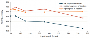
The number of inputs to the neural network is determined by how many bytes from each bidirectional flow is passed into the classifier. If the input length is too small then the classifier will be unable to detect patterns in the input, resulting in poor classification accuracies. As the input length increases, the degrees of freedom also increase, as shown in previous experiments this may lead to better accuracies.

To investigate this idea, three classifiers of varying degrees of freedom were trained on a series of input lengths ranging from 50 to 800 bytes. The classifier suffered no deterioration in the small input lengths, and therefore an input length of 50 bytes was be utilised for the subsequent experiments. This allowed for a reduced training time.

Training/Optimization Algorithm

The training algorithm (also called the optimisation algorithm) is responsible for minimising the cost function of the neural network. Adam [16] was the optimization algorithm used in all phases of this research due to its tolerance to ill-conditions and computation efficiency.

Threshold Function

The threshold function also known as the activation function is a function that is applied at every node in the NN. It is responsible for detecting non-linear patterns from the input. Rectified Linear Unit (ReLU) threshold function was used for all nodes in the neural network except those in the output layer. ReLU was chosen due to its fast computation performance and ability to accelerate convergence of gradient decent training algorithms. Softmax threshold function was used at the output layer because its output can be interpreted as raw probabilities.

Category Encoding

The number of nodes required for the input and output layers is determined by how the input and output categories are encoded. The network application classes and malicious classes are chosen to have no intrinsic ordering. Therefore, the value assigned to each output category does not matter as long as each value is unique. 1-of-C (sometimes referred to as “one-hot encoding”) is the most common encoding technique used for output encoding for a feed forward backpropagation neural network. 1-of-C encoding works by assigning each classification category a position in a vector. Each position in the vector is set to zero except for the corresponding output category.

Phase 2

The aim of this phase is to classify network traffic flows using extracted flow metadata from the packet captures. Unlike the other project phases which focus on detecting binary patterns inside the packets and data streams, this phase measures properties of each network flow for classification. For example, below is a list of some of the derived features that can be measured and used for network classification:

• Port number
• Total number of packets sent during a flow's lifetime
• Frequencies of packets sent from the client to the server
• Lifetime of the network flow

These network features can be automatically extracted from the network traffic using an exporter program and a collector program. An exporter collects low level flow information and formats it for the collector. The collector calculates high level features based on the flow information provided to it and then displays the result typically in a human readable format.

The testing accuracy as the input length is adjusted.

Chosen Feature Exporters

Maji and Tranalyzer were chosen as the main feature exporters based on their good classification results by Haddadi and Zincir-Heywood [17], and their compatibility with each other – both exporting features for uni-directional flows. This step was not performed in depth as it was expected that the deep learning model would automatically learn the most influential features, and be less affected by unimportant features.

Feature Extraction

Approximately 130 features were used in Phase 2 that were collected from two feature exporters. Only a minimal amount of research was put into the correlation of these features in regard to the network protocols and applications.

Feature Set Manipulation

Several features were then removed from the feature sets, as they were not relevant or were repeated. The features which were removed included:

• IPv4 addresses
• Internet Protocol Version 6 (IPv6) features
• MAC addresses
• ICMP related features
• First and last packet times in milliseconds and seconds

IPv4 addresses and MAC addresses were removed as they do not contain information that could contribute to classification outside of this data set. IPv6 features were discarded as the UNSW-NB15 data set did not contain any IPv6 packets. ICMP features were removed as we aimed to classify purely TCP and UDP flows. The first and last packet times were discarded because other features contained the packet times in microseconds, which were more accurate. After the removal of the features listed above, and the addition of two features which were provided with the ground truth labels – the bidirectional start and end times – 105 features remained.

Normalising Feature Data

To ensure each feature affects the neural network model fairly, and assist with convergence of the model, the input data was normalised to values between zero and one. This normalisation was based on the minimum and maximum of each numerical feature, and scaling the value linearly. Features which used strings were converted to a number using a pre-defined translation, and then scaled in a similar method to the numerical features.

Number of hidden layers

In the early stages of determining optimal model parameters, training was performed on 21 different models, and these tests indicated that a model with two hidden layers would offer the greatest testing accuracies and also keep computation time to a reasonable level, similar to the results of Phase 1. Subsequent tests therefore primarily used similar models.

Number of nodes in each layer

The number of nodes in the hidden layers were varied. For application and malicious traffic classification, using 500 nodes in both hidden layers proved effective. For malicious detection, a simpler model with 200 nodes in the first hidden layer and 30 nodes in the second hidden layer proved most effective.

Dropout

The training accuracy of the preliminary results was reaching significantly higher values than the testing and verification accuracies, and hence there was the possibility that overfitting was occurring. To gain optimal performance, a dropout stage was implemented after applying the activation function, which would encourage the use of more features rather than overdependence on a select few, as well as reducing overfitting.

Three configurations of dropout were tested. Each value represents the retention rates - the probability for which a node is retained:

• 0.5 in first hidden layer, 0.5 in subsequent hidden layers
• 0.85 in first hidden layer, 0.5 in subsequent hidden layers
• 0.95 in first hidden layer, 0.75 in subsequent hidden layers

The dropout retention rates which proved most effective were 0.85 and 0.5 for the first and second hidden layers respectively, which were used in subsequent training. This is based on an extensive application test, and an extensive malicious test in which the maximum accuracies were achieved using these dropout rates. This proved effective for some classification types and hence models were trained with and without dropout.

Selection of input features

The testing accuracy as the number of input features is reduced.

Another parameter that was adjusted was the selection of input features that the models trained with. As seen in Phase 1, reducing the number of input bytes from the first 1000 to the first 50 bytes resulted in similar results but require a less complex model. The effects of performing similar actions were therefore investigated in Phase 2. Additionally, by removing any features which did not contribute useful information to the output classification, the number of input features could potentially be decreased with no negative effects. To investigate this for Phase 2, the following investigations were proposed:

• Feature Selection: Removing input features based on the accuracies returned, training the model with the removed features, and continuing with the model with the highest validation accuracy.
• Random Feature Removal: Removing an individual input feature at random, training the model with this removed feature, and continuing by removing the next randomly selected feature.
• Individual investigation: Investigating each of the features, finding their relevance to the classifier and analysing the numeric or string values of each feature.

Due to the nature of this Phase, the removal of input features is less trivial than for Phase 1. Phase 1 found that the first 50 bytes could be used to train a model with a similar accuracy to using 1000 bytes. The basis behind this idea is that the most relevant data for classification is earlier in the flow. For Phase 2, however, the features extracted from Maji and Tranalyzer are in no order of relevance to classifying the flow, and alternative methods must be used to reduce the number of input features effectively. Method 1. Feature Selection unfortunately required many separate sequences of training which required an infeasible duration of training time. By limiting the input data set size and/or the number of epochs of training, the model could not produce results that accurately represented the potential of a fully trained model.

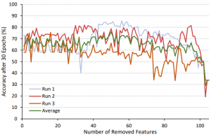
Method 2. Random Feature Removal was implemented for application protocol classification to give insight into the effects of random feature removal and the overall trends if less features were used in the data set. To reduce the required time taken to train each model, the input data set was reduced to 20% of the full size, and the number of epochs of training was limited to 30. Results would indicate whether the removal of features corresponds proportionally to a decrease in model accuracy.

Through Method 3. Individual investigation of the features it was found that some features were not relevant in description to the classification, and the numeric or string data for some features was redundant. The removal of some of these features helped improve testing classification accuracy in some models. Therefore, for subsequent training, two separated models were often trained – one set of training using all input features, and one set of training performed with the selection of features removed.

Phase 3

An overview of how data was arranged in an image.

The first two phases of this project have investigated the use of pre-existing network traffic techniques and how deep learning can be used to improve these methods. Phase 3 aimed to reverse this process. By evaluating the areas that deep learning is especially good at, Phase 3 investigated whether network traffic can be represented in a way such to utilise a method specifically designed for deep learning. CNNs are highly versatile networks that are able to search through a given input for features rather than evaluating the entire input at once; compared to a typical fully connected network, such as the one used in Phase 1 and 2, this allows a CNN to classify much larger inputs without drastically affecting the complexity and training time of the model. While most CNNs are commonly utilised for image classification, CNNs have shown promising results for other fields of research such as audio classification [18].

Data Set Generation

Particular research was put into how the data should be placed in an image. For a CNN to be an effective classifier the two input coordinates must have meaning. For example, the x and y coordinates of a picture relate to a spatial coordinate system, swapping any two rows or columns would reduce the quality of this picture. With this in the mind, the rows and columns of the generated image were made to emulate the progression of the flow. Each subsequent row of the generated image is a new packet in the flow, with the bytes contained in the respective packet filling out the columns. The colour of each individual pixel in the image is a greyscale colour which represents a single byte in the packet. As the dynamic range of greyscale varies from black (represented by the value 0) to white (represented by the value 255), this therefore becomes a one-to-one mapping with the 256-value range of a byte.

Produced image of a HTTP flow for Phase 3.

Confidence

Training a model to predict the correct output is desirable however also establishing a method to measure the confidence in the model’s prediction is useful for real world applications. Unfortunately, deep learning methods are offered viewed as black box algorithms due to the fact that studying their structure will not give any insights to how the output prediction was made. Instead model confidences in typically measured by observing the output prediction for a given input. Confidence values were estimated by measuring the difference between the two highest output predictions. Originally, the model confidence was estimated using the largest softmax output value as this would provide a bounded number between 0 and 1 however preliminary results showed that this was insufficient for entries with high confidence values. The higher confidence thresholds would converge to 1.0 for the majority of test cases.

It should be noted that measuring uncertainty just based of the NN output prediction can lead to poor results. For example, regions that are not well defined in the training set can result in undesirable high confidence in the output prediction. It was found that a NN will try to find an approximation function F that will separate the two classes A and B. Regions that have few or no training cases can result in artificially high confidence areas since the model is only updated when the output value is incorrect. This is only a concern if the training data set does not adequately represent the range of possible inputs values in the entire data set. The UNSW-NB15 data set contains over 1 million unique flows and therefore should be sufficient in size to not be affected significantly by this limitation.

Results

Phase 1

Application Classification

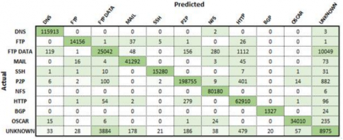
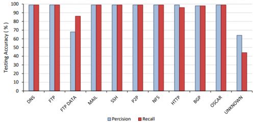
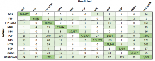
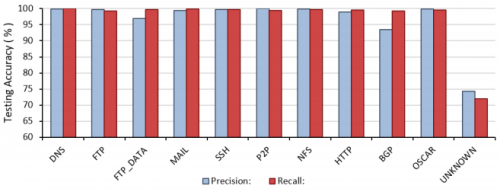
From the training process outlined previously, the performance of the model was then evaluated. Taking just under 50 hours to train, the classifier resulted in an overall classification accuracy of 96.9 % on the testing set. To examine the misidentified flows, a confusion matrix, and precision and recall graphs were constructed.

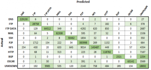
To examine the misidentified flows, a confusion matrix, and precision and recall graphs shown below were constructed. The confusion matrix shows that the vast majority of misclassified flows related to the unknown applications class. As this class was made up of a variety of unknown applications, it is expected that similar protocols may exist in the unknown class that could relate or even belong to the other applications. For example, the most significant difference was found to exist between FTP_DATA and unknown. Deri et al. [5] found that nDPI, a method used to add additional labels to this data set, had a FTP_DATA classification accuracy of below 75%. As the FTP_DATA flows not classified by this process would remain in the unknown category, there might exist a high enough quantity of FTP_DATA in the unknown class to confuse the classifier.

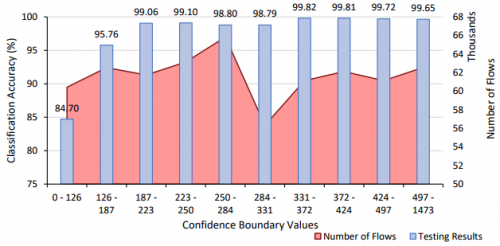
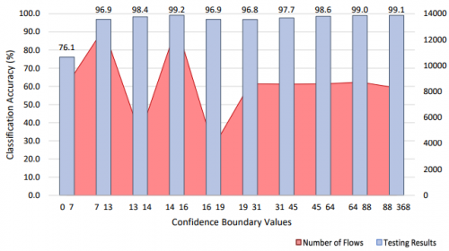
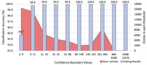
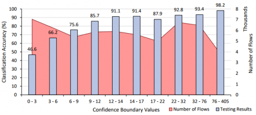
The confidence of each of the predictions was investigated. By taking the difference between the top two predicted classes of each input, we can see how confident the classifier is in making its prediction. A low value indicates that the model is finding it difficult to differentiate between two or more classes, whereas a high value indicates the level of confidence it has in classifying that input. Utilising this confidence level, a user can define a threshold at which point the classifier should or should not make a prediction for the current input. Non-classified inputs can then be identified through another method or by manual inspection. This level of confidence is a necessity when the cost of an incorrect prediction is high, such as miss identifying malicious traffic.

Malicious Traffic Classification

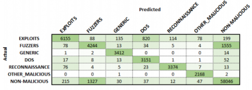
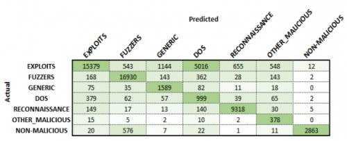
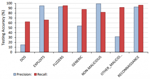
In a similar fashion to the application results, a classifier was then trained and evaluated over the malicious data set. The malicious classifier not only detected malicious activities but also had to classifying the type of malicious activity. Taking just over 22 hours to run, the malicious classifier achieved a classification accuracy of 94%. The confusion matrix, and precision and recall for the malicious classifier are shown below. It was found that the classifier was able to correctly identify most malicious classes, with the largest confusion occurring between non-malicious classes and a malicious attack known as a fuzzer. Fuzzers aim to probe the vulnerabilities in a network’s configuration by utilising a variety of different input values to try to break the programs allowable conditions. As these inputs are readily available to all users, a fuzzer attack can be hard to distinguish from a non-malicious flow when the context of the flow is not known. It is believed that this is this reason that the classifier is unable to reliably distinguish the two classes.

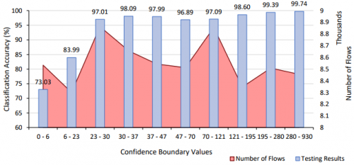
From the confidence graph it can be seen that by selecting only the predications with a high confidence, a very high malicious classification accuracy can be achieved. Increasing the confidence threshold also reduces the likelihood of false positives appearing which can be highly useful in practice if malicious activities have to be manually investigated after a positive result is detected.

Malicious Traffic Detection

Another set of results was evaluating the model’s performance as a malicious detector. This is similar to the malicious classifier but does not try to classify the specific malicious activity like the previous section showed. Classification accuracy of 96% was able to be achieved for the malicious detector in Phase 1. The confusion matrix shown below shows that the bottom left quadrant and the top right quadrant have approximately equal number of entries. As a result, the precision and recall values are approximately equal. The ratio of the number of malicious entries to non-malicious entries is approximately 1:2 (this holds for both the verification, testing and training data). Due to the fact the trained model has a slight bias towards classifying detecting malicious entries as non-malicious. This is a common issue for extremely skew data set such as the malicious traffic in the original UNSW-NB15 data set and can be fixed by further balancing the entries in the data set. The confidence graph shows as the confidence increases the classification accuracy increases until it reaches 99.1%.

Discussion and Outcomes

Achieving a classification accuracy of 96.9% for applications protocols and 94% for malicious classification, our results signify that deep learning can provide an effective and efficient method for the classification of general and malicious traffic. Although this phase was designed to validate the method from [1], due to the use of different data sets and classifier architectures, a direct comparison cannot be made. However, it was seen that similar results were achieved for the classes in which were common to the two investigations (HTTP, DNS, MAIL, P2P, and FTP).

• Two hidden layers were used to decrease training time while still meeting the complexity threshold.
• Padding flows that did not meet the required input length with zeros rather than random values resulted in a consistently higher classification accuracy.
• An input length of 50 bytes, instead of the 1000 used in Wang (2015), granted an increased classification accuracy and a reduction in the training time for the used data

set.

• It is speculated that given a more extensive data set, the classification accuracies couldbe improved on and extrapolated onto a wider range of network traffic protocols.

Phase 2

Application Classification

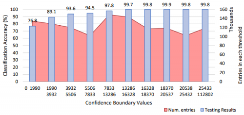
Training was performed using the full data set for approximately 200 epochs. The highest verification accuracy was achieved after 34 epochs, which corresponded with the highest testing accuracy of 94.9%. The confusion matrix and precision and recall for this model are shown in Figure 30 and Figure 31 respectfully. Similar to Phase 1, the largest discernible error is UNKNOWN being predicted as FTP-DATA. This may again be due to the inaccuracies associate with labelling using nDPI [5]. As observed in the confusion matrix, BGP was often misclassified as UNKNOWN, and as discussed for Phase 1, this may be due to the UNKNOWN class containing a proportion of BGP flows. A clear trend can be observed in the confidence graph that indicates a higher confidence value corresponds to a higher classification accuracy. For scenarios where an accuracy above 99.7% is required, only results with a confidence threshold greater than 13286 could be considered.

Malicious Traffic Classification

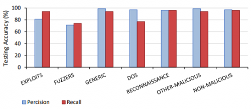
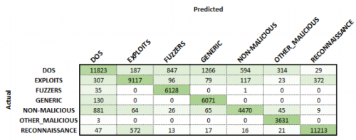
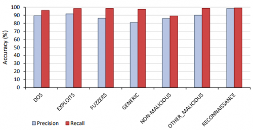
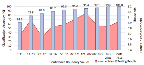
Training was performed for a total of 30,000 epochs resulting in a training time of three and a half days. The maximum verification accuracy was obtained at epoch 19,919 with a corresponding testing accuracy of 89.53%. The confusion matrix shows that a high proportion of NON-MALICIOUS flows were classified inaccurately as DOS. This may be due to the nature of a DOS attack, which involves repeatedly generating non-malicious traffic to overwhelm a network. As seen in the precision and recall graph however, the Phase 2 malicious classifier had particularly poor precision for the GENERIC class, and poor precision and recall for the NON-MALICIOUS class. Both of these classes are combinations of different types of classes, and hence may be difficult to classify. The recall of other classes, however, is generally quite high at 97% or above, which indicates there were only a small number of cases where other classes were incorrectly labelled as these. As shown in Figure 35, there is a strong relation between confidence and classification accuracy, and hence if required, the confidence level could be used to specify a lower boundary of accuracy.

Malicious Traffic Detection

The results for this classifier indicated an increased performance in classification between malicious and non-malicious traffic over the general malicious classification model. Training was performed for a total of 5000 epochs which took one and a half days. The best verification accuracy occurred at 2688 epochs resulting in a testing accuracy of 98.44%. As shown in the confusion matrix, most flows were correctly identified as malicious or non-malicious. It is again observed that a lower confidence indicated a reduced accuracy, but most entries occurred in lower confidence boundaries, as opposed to more even distributions seen for other models.

Discussion and Outcomes

This phase investigated the viability of deep learning for network traffic classification in a different approach to Phase 1. Phase 1 relies on a combination of header data and payload data, and while it achieved excellent results, this reliance may fail due encryption of the payload. Phase 2 has demonstrated that this reliance on the payload data is not required to achieve accurate results, and opens the possibility of classifying encrypted data. Throughout this phase, the optimal parameters were determined and are described for the best application, malicious classification and the malicious detection models. Results indicated that using dropout was effective for application and malicious detection results, and that using two hidden layers returned best results for all classification types. Similarly to Phase 1, higher complexity models offered negligible benefits to the classification accuracies. The application classification results compare similarly to the work by Auld et al. [3], which used Bayesian Neural Networks and testing and training data recorded eight months apart. They achieved an accuracy of 95.8% with over 200 features, and 93.6% with 65 features. In comparison, Phase 2 achieved an accuracy of 94.9% using a set of 105 features, and an accuracy of 92.3% using 55 arbitrarily chosen features. The results gathered by Auld et al. [3] and within this phase indicate that by using additional features would likely improve this classifier. Further improvements could be made with the use of a more complete data set, as ground truth labels were not provided for a large proportion of flows. This may have had a particular influence on the classification of the UNKNOWN class for application classification, hence reducing the overall accuracy.

Phase 3

Application Classification

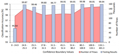
Taking just under 30 hours to train, the classifier resulted in an overall classification accuracy of 99.5% on the testing set, an improvement on both Phase 1 and 2. The misidentified flows and classification accuracies of each class were then examined using Figure 50 and Figure 51. While Phase 3 still suffers from the major sources of misclassification identified in Phase 1 and 2, the severity of these areas has been drastically reduced. Through the process described in Phase 1, a confidence graph of the application results was then constructed. As shown in below, it was found that all bins except the lowest confident bin achieves a classification accuracy of above 99%. Therefore, defining a confidence threshold of 24.9 would result in classification of approximately 100% while only 9% of the data set would remain unclassified.

Malicious Traffic Classification

Training for 24 hours, the malicious classifier achieved an overall classification accuracy of 81.5%. From the confusion matrix and precision and recall graphs shown below, the misclassified flows can be identified. It was seen that the largest source of confusion occurred between the malicious class EXPLOITS and the remaining malicious classes. While not to the same extent, this result was seen in both Phase 1 and 2. Exploits are used to ‘exploit’ the vulnerabilities on a system to enable the execution of code to either corrupt or further spread the malicious intent. As this type of malicious attack can vary significantly depending on purpose and location of attack, it is seen that the classifier cannot reliably correlate this variation. As this phase only used two thousand samples for training this class, it is theorised that a more extensive data set could improve these results

Malicious Traffic Detection

However, a reasonable estimate can still be gained through the summation of the malicious classes in the previous test. It is shown that the malicious detection accuracy correctly identified 98.9% of the malicious samples as malicious. While the classification accuracy of the individual malicious classes is reduced compare to the previous phases, its ability to identify malicious samples has improved. However, it should be noted that the classifier is more ‘cautious’ than the previous phases, identifying a higher proportion of non-malicious classes as malicious. This result is speculated to have occurred due to the reduction of non-malicious samples used within the training set. As this phase required the training set to be evenly distributed, the reduction in non-malicious training samples resulted in the total number of malicious classes dominating the training.

Discussion and Outcomes

This phase investigated the use of a deep learning method that is commonly reserved for image based classification.

Through the investigation of different architectures and hyperparameters, a highly accurate classifier was developed. While not achieving the same classification accuracies as the other two phases for malicious traffic, it was found that this phase proved a superior classifier for the application classes. From analysing the confidence of the Phase 3 classifier on the application testing set, it was found the classifier could approach a classification accuracy of 100% for over 90% of the testing set.

Conclusions and Future Work

Conclusions

Through the construction and exploration of three distinct deep learning classifiers, we have shown that deep learning is a viable solution for network traffic classification. We have found that representing this traffic in the form of byte sequences, as for Phase 1, or images, as for Phase 3, both allow for highly accurate classification. The completion of Phase 1 demonstrated that the work by Wang [1] could be performed on an alternative data set. Phase 2 performed comparatively to the work by Auld et al. [3] which used extracted features from an alternative data set, however using Bayesian Neural Networks. Phase 3 focused on the innovative approach of using Convolutional Neural Networks and demonstrated that it was capable of producing excellent classification results.

Additionally, an approach to calculating the confidence of a result was implemented for each phase and shown to have a clear relationship with the output accuracies, thus allowing for the predicted accuracy of a particular result. In particular, it was shown that:

• The input method presented by Wang [1], was validated on the UNSW-NB15 data set, achieving a classification accuracy 97.5% on the used data set. Furthermore, it was found that this method could be extended to the use of classifying malicious traffic, with a resulting classification accuracy of 94.2%.
• Statistical features of the flow can be used as input features to deep neural network, albeit with a slightly diminished classification accuracy.
• An image based classification of network traffic is an effective way to classify application traffic, with 100% classification accuracy for over 90% of the testing data set.
• A confidence threshold could be utilised to indicate the flows in which the classifier is unsure of. This ability could be used to create a more accurate classifier by reducing the number of false positives, and is useful to a wide range of domains.

Future Work

Deep learning is an extensive field with an unbound number of uses. In this report we have only scratched the surface of the potential utilisation of deep learning for network traffic classification. A few examples of future work that could be used to extend this investigation are given below:

• Unsupervised learning could be investigated on unlabelled data to see the performance of deep learning clustering methods.
• Although the methods explored in this report were theorised to work with encrypted traffic, this was not tested. As the amount of encrypted traffic on a given network is rapidly increasingly, classifiers robust to different encryption methods are of high interest.
• Due to the complexity of the classifier, it is theorised that deep learning could detect and classify flows based on a variety of different outputs such as originating operating system or location.

References

[1] Z. Wang, "The Applications of Deep Learning on Traffic Identification," Black Hat USA, 2015.

[2] S. Zeba and D.G. Harkut, "An overview of network traffic classification methods," International Journal on Recent and Innovation Trends in Computing and Communication (IJRITCC), no. ISSN: 2321-8169, pp. 482 - 488, February 2015.

[3] T. Auld, A. W. Moore, and S. F. Gull, "Bayesian neural networks for internet traffic classification," IEEE Transactions on Neural Networks, vol. 18, no. 1, pp. 223-39, Jan 2007.

[4] A. W. Moore and K. Papagiannaki, "Toward the Accurate Identification of Network Applications," in PAM, 2005, vol. 5, pp. 41-54: Springer. An intensive examination of network traffic and methods to classify them.

[5] L. Deri, M. Martinelli, T. Bujlow, and A. Cardigliano, "nDPI: Open-source high-speed deep packet inspection," in 2014 International Wireless Communications and Mobile Computing Conference (IWCMC), 2014, pp. 617-622. A deep packet inspection tool utilise to add additional labels to the UNSW-NB15 data set.

[6] V. Carela-Español, P. Barlet-Ros, A. Cabellos-Aparicio, and J. Solé-Pareta, "Analysis of the impact of sampling on NetFlow traffic classification," Computer Networks, vol. 55, no. 5, pp. 1083-1099, 2011. The “UPC” data set, used by both the 2014 and 2016 iterations of this project.

[7] B. McAleer et al., "Honours Project 10: Development of Machine Learning Techniques for Analysing Network Communications," The University of Adelaide, Adelaide 2014. 2014’s iteration of the project. Investigated network traffic with tree based and SVM classifiers.

[8] K. Hörnlund, J. Trann, H. G. Chew, C. C. Lim, and A. Cheng, "Classifying Internet Applications and Detecting Malicious Traffic from Network Communications," ECMS, The University of Adelaide, 2016. Last years’ iteration of the project. Explored network traffic classification utilising graph based techniques.

[9] C. Trivedi, M.-Y. Chow, A. A. Nilsson, and H. J. Trussell, "Classification of Internet traffic using artificial neural networks," 2002. Used the packet size for classification. Showed a neural network was favourable compared to a standarised clusting technique.

[10] J. Quittek, T. Zseby, B. Claise, and S. Zander, "Requirements for IP Flow Information Export (IPFIX)," Internet Engineering Task Force. (IETF), October 2004. Used to understand the requirements for IPFIX designation.

[11] A. Ng. Machine Learning. Available: https://www.coursera.org/browse/datascience/machine-learning A free course on machine learning. Was used initially to get fimilar with the concepts.

[12] Neural Network FAQ. Available: ftp://ftp.sas.com/pub/neural/FAQ.html An extensive resource for information reagarding neural networks.

[13] J. Rajagopal, I. Descutner, M. Scibior, and N. Pickorita. (2016). Deep Learning SIMPLIFIED. Available: https://www.youtube.com/watch?v=iIjtgrjgAug A YouTube series, useful to get fimilar with the different deep learning networks.

[14] A. Martín et al., "TensorFlow: A System for Large-Scale Machine Learning," in OSDI, 2016, vol. 16, pp. 265-283. A python library utilised to create and evaluate all models used within this project.

[15] M. Nour and J. Slay, "UNSW-NB15: a comprehensive data set for network intrusion detection systems (UNSW-NB15 network data set)." Military Communications and Information Systems Conference (MilCIS), 2015. IEEE The data set used for all experiments shown in the report.

[16] D. Kingma and J. Ba, "Adam: A method for stochastic optimization," 2014. The optimisation algorithm used for all classifiers in this project.

[17] F. Haddadi and A. N. Zincir-Heywood, "Benchmarking the Effect of Flow Exporters and Protocol Filters on Botnet Traffic Classification," IEEE Systems Journal, vol. 10, no. 4, pp. 1390- 1401, 2016. Showed a comparison between available feature extraction tools. Was used to decided which tools to use in Phase 2.

[18] S. Hershey et al., "CNN architectures for large-scale audio classification," in 2017 IEEE International Conference on Acoustics, Speech and Signal Processing (ICASSP), 2017, pp. 131- 135. Showcases other uses for CNN architectures. Inspiration for Phase 3.

[19] C. Szegedy, V. Vanhoucke, S. Ioffe, J. Shlens, and Z. Wojna, "Rethinking the inception architecture for computer vision," in Proceedings of the IEEE Conference on Computer Vision and Pattern Recognition, 2016, pp. 2818-2826. Showed that addition of multiple CNN layers could reduce the training time of a CNN classifier with large window sizes.