Projects:2018s1-101 Classification of Network Traffic Flows using Deep and Transfer Learning

Team

Students

Jack Baxter

Robert McAuley

Mitchell Mickan

Supervisors

Dr Hong-Gunn Chew

Dr Adriel Cheng (DST Group)

Mister Dr Kyle Millar

Introduction

Network traffic classification is useful for areas such as network management, traffic analysis and malicious threat detection. Traffic classification allows prioritisation of time-sensitive data (e.g. Voice over IP, Video Conferencing, Stock Market Trading) which can result in a better user experience. It can also help with understanding network trends and user patterns [38]. Threat detection can also have huge implications for network security.

The paper "Outside the Closed World" [38] discusses the large divide between commercially deployed intrusion detection systems and techniques in public research. Many commercial systems use signature-based detectors to alert when an attack is underway. However, these systems rely on a human developed signature and do not generalise to new attacks. In contrast to commercial systems, research has been traditionally focused on machine learning techniques and more recently on deep learning [38].

Machine learning has the ability to learn underlying complex relationships that aren't explicitly obvious to a human. Machine learning models learn general patterns, as opposed to specific signatures. With the increase in the availability of big data and increases in computing power, deep learning, a subset of machine learning, has become popular. Since 2012 deep learning has been credited with large advances in natural language processing, computer vision and pattern matching tasks [2].

Following success in other fields, deep learning has been researched for use in the field of network traffic classification. An important goal for deep learning models is to work on networks beyond those it was trained on. This concept is called 'Generalisation'. In addition, we want these models to learn patterns representing general malicious activity and be able to detect previously unseen attacks. However, due to the lack of availability of good datasets, progress has been slow [38][2].

Due to the large amount of data flowing through networks, it is time-consuming and often impractical to manually label a network traffic dataset. Additionally, there are privacy concerns with publishing packet captures that have been collected from public networks [38]. Synthetically generated datasets are often used as an alternative, however, they are not always representative of real-world traffic. A model that displays good generalisation would help combat this issue due to it being able to label new data.

However, creating a network traffic classifier that generalises well is a difficult problem to solve. This is because network traffic can vary greatly from one network to another. In addition, the traffic patterns can also vary over time. Because of this, patterns and relationships learnt from one network do not necessarily apply to another network, nor do they necessarily apply at different points in time. Therefore it is important for a network traffic classifier to be able to generalise to data it has not been trained on.

There are techniques for improving the generalisation of deep learning models by taking advantage of previously learnt knowledge. The broad category for these techniques is known as transfer learning [28][29][41]. As far as we can tell, there has not been previous research exploring the generalisation performance of deep learning models for network traffic classification.

Previous work by honours students at the University of Adelaide [21] in 2017[1] has demonstrated the viability of deep learning models for network traffic classification. We aim to build upon this work by exploring the generalisation of these models and whether transfer learning techniques provide improvement.

Relevant Work

The section covers related work in the areas of network traffic classification, transfer learning, and network traffic datasets.

Network Traffic Classification

Network traffic classification is a broad field, often applying machine learning techniques. It is the study of computer networks and how to obtain information about those networks. Some of the typical problems in this field involve application detection, malicious actor and traffic detection, malicious traffic classification, network configuration detection, and device detection. Classification in this context refers to "What type of traffic is this?" whereas detection refers to "Is this type of traffic present?".

Prior to 2017, many methods for packet and flow classification did not use deep learning, instead using classical techniques. A survey by Garcia et al. [11] in 2014 reviewed techniques for botnet detection. The techniques surveyed had a focus on anomaly detection and used heuristic-based (or rule-based) methods. These methods require careful tuning before they can achieve good performance [11].

During 2017, there were a few papers that investigated the viability of deep learning techniques. Compared to classical techniques, deep learning techniques reduce the amount of manual heuristic analysis by automatically learning them from the data. Previous work done at the University of Adelaide in 2017 [21] used deep learning techniques for application traffic classification, malicious traffic detection and malicious traffic classification. The paper explores model performance using three different kinds of network traffic data: packet payload data, flow statistics, and entire packets. Flow statistics are statistics computed over packets in that flow, as opposed to pure packet data.

On the task of website fingerprinting (what websites are traffic connecting to), Oh et al. [26] showed in 2017 that deep neural networks can be used to classify website traffic with 99% accuracy. Within the context of application classification, neural network techniques have been shown to achieve high accuracy in detecting many common types of application traffic. The paper by Lotfollahi et al. [24] uses a deep convolutional neural network to classify application traffic with 97% accuracy.

Some related work uses flow statistics for network traffic flow classification. For example the paper by Ang et al. [23] achieved 99% classification accuracy using flow statistics. Another paper by Lopez-Martin et al. [3] achieved an application flow classification accuracy of 96.3%.

Transfer Learning

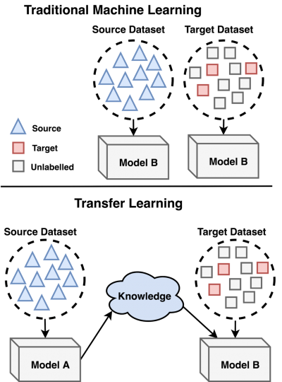
Transfer learning is a field in machine learning which looks at using knowledge learned from one task to achieve better performance in another task. Utilising transfer learning was the main objective for this project, with research conducted into various techniques and their suitability.

Pan et al. [30] (2010) and Weiss et al. [41] (2016) present surveys of transfer learning techniques. These papers highlight many different techniques for transfer learning and their relative performance in different domains. Homogeneous and heterogeneous transfer learning techniques were explored. Homogeneous refers to transferring knowledge to a domain with a similar feature space while heterogeneous refers to transferring knowledge to a different feature space. Network traffic has similar types of features (packets) so this work is more concerned with homogeneous transfer learning techniques.

Most methods presented attempt to correct the marginal or conditional distribution differences between the source and target. This can be done symmetrically by bringing both distributions together, or asymmetrically where one distribution is adapted to match the other. In most cases conditional distribution matching could only be achieved with some labels in the target space or by generating fake labels using the learner from the source domain.

One method that matches the conditional and marginal distributions is called CP-MDA by Chattopadhyay et al. [7]. The downside of their method was that it required multiple labelled sources, which makes it more difficult for testing. Another technique that attempts to bring the marginal distributions together was proposed by Daume et al. [19], through duplication of features. Joint Domain Adaptation by Long et al. [22] uses dimensionality reduction and pseudo labels of the target domain to adapt the conditional and marginal distributions of the source and target. Another method by Glorot et al. [16] looked at using Autoencoders to encode features into a different feature space and learning on the transformed features. Target features are then passed into the Autoencoder before being classified by the original learner.

Other techniques for transfer learning looked at finding the latent features that represent both the target and source domains. These latent features could be used to train a learner that could theoretically perform well in both domains. Some techniques that used this approach included work by Pan et al. [29], Gong et al. [17], and Shi et al. [36]. Another approach by Pan et al. [28] also suggests a technique that not only looks to find the latent features but attempts to align the non-latent features so that they can be used as bridge for knowledge transfer.

Some other techniques found do not fall into the previously mentioned categories. This included an adaptive layer technique proposed by Oquab et al. [27]. This method suggested training on the source domain and then freezing all layers of the model except the last. The last layer is then trained on a small amount of data from the target domain. Ideally this layer adapts differences in conditional and marginal distributions. The downside of this method is that it requires some labelled target data. The method by Gharibshah et al. [14] uses a pseudo labelling method to generate a new model. The original model is applied to the target and predictions with high confidence are taken as truth. This forms a pseudo labelled target dataset in which a new model can be trained on.

Datasets

To create a good classifier, a large amount of good quality training data is necessary. Multiple datasets are also needed for the purposes of testing transfer learning and generalisation. While preferably a system could learn using real world data, obtaining ground truth labels is a difficult and expensive task [38]. Additionally, there are privacy issues related to releasing real network data as a publicly available dataset [38]. Hence, many datasets are synthetically generated in a simulated environment. It is important that these datasets are realistic so that a classifier trained on them can generalise effectively to real world systems (inter-domain generalisation). This includes having realistic non-malicious traffic and malicious attacks in the dataset.

One of the main datasets used in this project was UNSW-NB15 [25]. This was the dataset used in previous years work [21]. It is a synthetically generated dataset created specifically for the task of evaluating Network Intrusion Detection Systems (NIDS). The dataset contains both malicious and non-malicious traffic that was generated by an IXIA traffic generator placed in a simulated network. In total the dataset contains approximately 100GB of raw packets and labeled flow data collected over a period of two days.

Another useful dataset is the CICIDS dataset [35][13] created by the University of New Brunswick. This is a more recent dataset that aims to contain up to date traffic and current attacks. It contains around 51GB of raw packet data collected over a simulation period of 5 days. Different categories of attacks are executed on different days.

Previously, the University of New Brunswick released another Intrusion Detection dataset in 2012 - the ISCXIDS dataset [37]. It is similar in format to the newer CICIDS dataset, containing around 85 GB of packet data spread over a simulation period of 7 days with different attack categories. The reasons given by the authors of CICIDS for creating an updated data set was that the ISXCIDS dataset no longer represented current trends of real networks as it did not contain any form of HTTPS traffic.

Besides general intrusion detection datasets, the University of New Brunswick have released several other datasets for more specific tasks. These include datasets that contain Virtual Private Network (VPN) and non-VPN traffic, Botnets, Android Botnets, Tor and non-Tor traffic, DoS attacks, and Android Adware.

Another dataset is the CTU-13 dataset [12] which focuses on malicious data coming from botnets. This is data collected from a network that contains a series of virtual machines that have been infected with real botnet malware. These virtual machines are connected to the internet and bridged with a university network, where background data is collected from real users. 13 different scenarios are created with different kinds of botnets. The malicious data is published as raw packet data (PCAP) while non-malicious data is published as labeled netflow files.

There are other datasets such as the Booters dataset [34] which focus on providing labelled data of DDoS traffic. In this dataset, the authors use online services called Booters that provide DDoS as a service, to purposefully attack their own controlled network and capture the data. The data received from each separate service are released as raw packet captures.

Some datasets focus on application fingerprinting. One such dataset is the Universitat Politecnica de Catalunya (UPC) dataset. The UPC dataset contains 600GB of captured packets with labels detailing the associated application [6].

Background

Network Traffic

In a computer network, data is exchanged between computers and servers in the form of network packets. Network packets contain not just user data, but several layers of control data which are added, removed or otherwise modified as the packet travels on the way to its destination. The part of a packet that contains the control data is called the header, while the actual message data is called the payload.

Computers, servers and routers in a network are collectively referred to as 'network nodes'. A network 'flow' refers to a series of packets that are all part of the same conversation between two network nodes. All of the packets within the same conversation, a network flow, are defined by the same five fields (referred to in this thesis as a 5-tuple key):

• Destination IP address
• Source IP address
• Destination Port address
• Source Port address
• Transport Protocol (e.g. TCP, UDP)

A unidirectional flow means traffic flows in a single direction from one node to another. A bidirectional flow is all the traffic that flows in either direction between two nodes.

Network Attacks

In a computer network, attacks arise in many different forms. Malware refers to any form of malicious software that carries out unwanted activity. There are further sub classifications of malware such as viruses, worms and botnets that differ slightly in their behaviour. Network attacks can be carried out by malware or by entities outside a network. The list below details some attacks and their definitions.

• Exploits: Any kind of attack that relies on exploiting bugs in existing software, from which malware can be installed or run.
• Denial of Service (DoS) & Any form of attack that attempts to prevent legitimate user from accessing the network or services.
• Distributed Denial of Service attack (DDoS): A DoS carried out by many machines, often due to being infected by a Botnet.
• Fuzzers: Any form of attack which attempt to find new exploits / vulnerabilities by attempting many different combinations of inputs.

Machine Learning

Machine learning is the name given to the development of computing systems that use data to become progressively better at a task. Tasks can refer to any number of problem categories such as prediction, classification, clustering, forecasting and association discovery. Prediction and forecasting is where a machine learning system makes an inference about some state. This can include things like server utilisation prediction, stock market trends, housing prices, vehicle traffic flow and many others. Classification, clustering and association discovery fall under a different objective, categorisation. Some examples are: determining what objects are in an image (classification), determining groupings of users based on their interactions (clustering), and discovering regularities in products sold in online marketplaces (association discovery).

The systems that make predictions are typically called models. Models are made up of a collection of parameters (learned values) arranged in a way to transform input data from one form to another.

Model Generalisation

Model training can be defined as the process that captures the underlying marginal and conditional distributions in the data. The model should capture these distributions on a global scale, learning the general distributions for the problem rather than those specific to the dataset. For example, if a classifier is trained to classify malicious traffic on one network ideally it also works on another network. A model is said to generalise when it achieves good performance on data outside of the training data. There are two main types of generalisation: intra-domain and inter-domain generalisation.

Intra-domain Generalisation

Intra-domain generalisation refers to the ability for a model to generalise well within the domain it learnt from. In other words, how well the model understands the probability distributions within a single dataset. This performance can be seen by splitting the dataset into two sections, called the train set and the test set. When training, the model only uses data from the train set. If the model has similar performance on both test and train sets then it can be said that it has good intra-domain generalisation. If the model achieves very good performance on the train set and poor performance on the test set then the model is said to be 'overfitting'. This means the model is learning an overly complicated trend that represents the train set well but does not necessarily fit the test set.

Inter-domain Generalisation

Inter-domain generalisation refers to the ability for a model to generalise well to new datasets outside of the one it learnt from. Given a problem, it is assumed that there is some underlying probability distribution describing all possible samples within the domain. By investigating inter-domain generalisation performance, this enables gathering of evidence as to whether the model is learning the global underlying probability distribution. If the performance is poor the model may be overfitting and only learning to match the training data. Another possibility is that the training data isn't a good representation of the problem. An example of good inter-domain generalisation would be a model with the ability to achieve similar classification performance on traffic from a different network to the one it was trained on.

Transfer Learning

Transfer learning is an area of machine learning that looks at applying knowledge gained from one problem or domain and applying it to another. Certain problems utilise knowledge that can be useful in other tasks, e.g an image classifier that classifies cars may contain knowledge that is useful for classifying other vehicles.

The source domain is defined as the domain in which training was done and the target domain as the domain in which knowledge is transferred to. If the source and target domain have the same feature space (type of input is the same) then it is called homogeneous transfer learning. If they are different it is called heterogeneous transfer learning.

Deep Learning Models

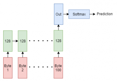
We extended/reproduced the models from [2]. Additionally, we proposed using a Multicell Recurrent Neural Network with Long Short Term Memory cells.

Recurrent neural networks (RNN) are typically useful for time series or data that has a sequential nature to it. These aspects could be useful for several reasons. Firstly at the packet level the bytes of a packet are interpreted sequentially with data often spanning over multiple bytes. For example the 'Total Length' field of an IPv4 header spans two bytes and can be better interpreted by a network when looking at both together. An RNN with its ability to store the state of previous features may be more likely to properly interpret the full field than other deep learning networks.

Validation of Concept

To evaluate the performance of a Recurrent Neural Network, we trained it on both the biased and unbiased datasets, measuring test set accuracy.

	Biased Dataset (%)	Unbiased Dataset (%)
Overall Accuracy	99.2	99.1
Average Class Accuracy	91.2	91.5

This model achieves very high single class accuracy across all classes. Interestingly the biased and unbiased models do not differ that much. The main benefit of the unbiased model is that it will not depend on the biased fields when applying to a new dataset. Already we see that we can get very high average class accuracies for packet classifier at 91.2% average class accuracy compared to [21][3] which had 83.0% for their 2D CNN. The only flaw in this comparison is this model classifies packets while theirs classifies flows.

Transfer Learning Techniques

Our project explores five different transfer learning techniques and applies them to the problem of network traffic classification. Their performance is compared against various baselines to see how much improvement they offer.

Naive Technique

Background

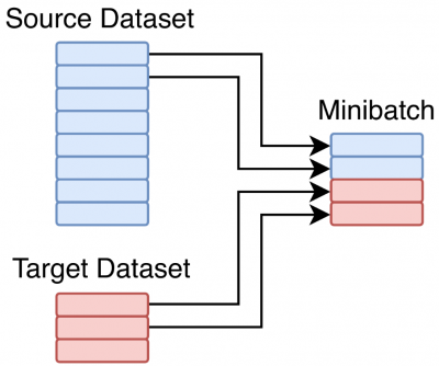
The Naive Model is a method which combines data from a source and target dataset. A model is then trained on this data, without using any other transfer learning technique.

The Naive Model doesn't extend the model architectures but instead modifies the training data to instead train on the union of the source and target datasets. Given a source and target dataset the model will fill minibatches half with data from source, and half data from target. If one dataset is smaller than the other, the smaller dataset will start repeating before the other. This is effectively equivalent to oversampling the smaller dataset until it equals the size of the larger dataset. The daigram below shows this process with a target dataset which is much smaller than the source.

Findings

The table below shows the averages of improvements for different classes across all models using the naive method.

Experiment	Average Improvement
Binary Packet	7.06%
Multiclass Packet	0.81%
Binary Flow	6.14%
Multiclass Flow	0.53%

The results indicate that the naive method is able to achieve high positive transfer for binary classification, increasing average class accuracy by an average of 6.6%. The technique does not perform as well on multiclass classification where results show on average an insignificant increase of 0.67% in performance. In the multiclass setting, the technique is effective for the ISCXIDS to CICIDS datasets but is only harmful for the UNSW-NB15 to CICIDS datasets.

Frustratingly Easy Domain Adaption

Background

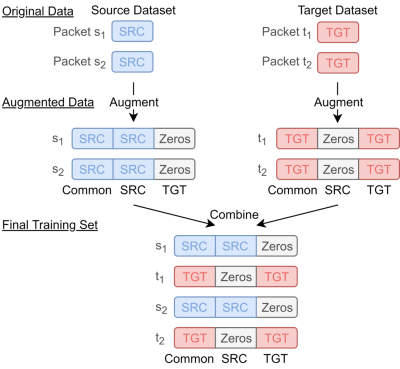
Another transfer learning technique we consider is Frustratingly Easy Domain Adaptation (FEDA) proposed by Daume et al. [19]. It is an asymmetric transformation technique that augments the source and target datasets by creating duplicates of the original features. The technique is shown to be effective for natural language processing tasks when training with only target data is slightly more effective then training with only source data [19].

The FEDA transformation technique as described in [19] augments the source and target datasets by creating three versions of the original features. The three versions are the general version, source-specific version and the target-specific version. In the augmented dataset, data from the source domain will contain the general and source-specific versions. Data from the target domain will contain the general and target-specific versions. This augmented dataset is then used for training the model. A diagram of the augmentation process is shown below.

When a learning algorithm trains on the augmented dataset, it chooses features from either the common, source, or target feature set. For features that provide a good classification across both target and source domains, the common feature set is preferred. For features that provide a good classification in the source domain but do not generalise to the target domain, the source feature set is preferred. For features that provide good classification in the target domain but are not useful in the source domain, the target feature set is preferred. The feature set choices are not done by any specific algorithm but result as a consequence of model training. I.e. During training, the model learns the best features to use.

Findings

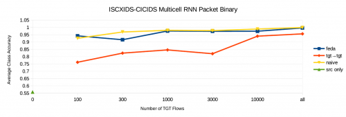
The graph below shows an example of the performance using FEDA versus the Naive model and target only training at a variety of reduced target dataset sizes

These experiments show that Frustratingly Easy Domain Adaptation can improve performance over target only training for RNN models with an average improvement of 4.78% in average class accuracy. It is however not effective for CNN models resulting in a slight loss of performance when applied to these models.

The technique also does not perform better than the Naive model in most cases, with an average -0.72% loss of average class accuracy.

Adaptive Layer

Background

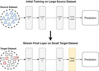
Another technique explored is the Adaptive Layer technique introduced by Oquab et al. [27]. This technique leverages an existing model, adapting the final layer to the new dataset. Originally it was used for computer vision, with the idea that many image classifiers learnsimilar low level features and the final layers interpretation of them is the main difference.Adaptive Layer was explored for network traffic classification as the core structure of a packetor flow doesn’t change across datasets. This lead us to believe that this technique may be applicable.

The Adaptive Layer technique assumes we have a small amount of labelled target data. Initially a deep learning model is trained on only the source dataset. The final layer of this model is then retrained using the small amount of target data. All the other layers are leftas they were when trained on the source dataset. A diagram showing how this techniqueworks can be seen below.

Conclusion

We find that the adaptive layer technique is not effective for improving the target performance when we have one of our models trained on a source dataset and a small amount of target data. Training a model from scratch using the small amount of target data provides higher performance than applying this technique. Further research into this technique could utilise a larger pretrained, proven network traffic classifier. This would provide a scenario more similar to the original paper and may provide better results.

Cross Seeding

Background

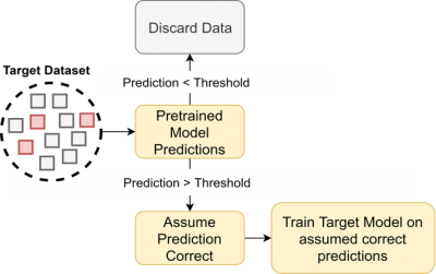
Cross Seeding is a technique taken from [14] by Gharibshah et al. Cross Seeding was origi-nally developed to identify and classify IP addresses from online forums. This technique canbe applied to a variety of different problems due to it only requiring a source model and anunlabelled target dataset. For this reason, it’s application to transfer learning for networktraffic classification was tested.

Cross Seeding aims to improve performance on a target dataset when the target dataset is unlabelled. The technique assumes we have a labelled source datasetand a model trained on this dataset. Cross seeding also doesn’t require any labelled targetdata. This is one of the main benefits compared to other techniques which often requiresome labelled target data.

When Cross Seeding a model trained on the source dataset is applied to the unlabelled targetdataset. High confidence predictions are taken as true, and retained as labels for the target.Although some target labels may be incorrect, most should be correct due to the predictionsbeing high confidence. A diagram showing this technique can be seen in below.

Findings

Cross seeding is effective at providing a small boost for malicious traffic classification on atarget dataset when using a model that has been pretrained on a labelled source dataset. We note on average a 2.8% improvement of average class accuracy for binary models and 6.6% for multiclass models. We also conclude that Cross Seeding is more effective the poorer the target performance is.

We find that our Adaptive Threshold Cross Seeding method results in a more even distribution of labels which allows us to train better target models. Our adapted technique gives an average of 4.7% improvement compared to the 0.7% of the original technique. The downside of this method is that we must specify the number of labels to take as anotherhyperparameter.

Our results indicate that our malicious network traffic classification modelscorrectly learn the representation for non-malicious traffic. They also provide evidence that these models heavily overfit to the various malicious classes.

Stacked Autoencoders

Background

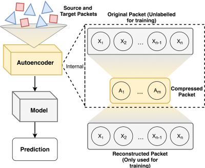
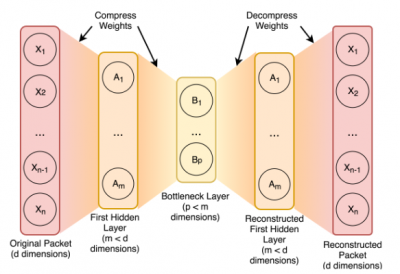
An Autoencoder is a model that learns to encode (or compress) an input to a lower dimensional space while retaining the ability to decode (or decompress) back to an output. The goal is for the reconstructed output to match the input as closely as possible. Glorot et al. [16] proposed an adaptation that allows Autoencoders to be used for transfer learning. Their formulation uses a Stacked Denoising Autoencoder to transform source and target data into a common representation. Learning this transformation allows an Autoencoder to resolve the marginal distribution differences between the source and target datasets. Samples from either dataset (source or target) can then be transformed, via the Autoencoder, into a compressed representation which is used to train a classification model. The act of learning a transformation from both the source and target datasets allows a Stacked Autoencoder to create a common representation and accomplish transfer learning.

Single-layer Autoencoders take an example packet X from the input dataset, compress it to dimension m, and then decompress it back to dimension d (See first figure in this section). The output represents a reconstructed packet. To train the weights of the network, Root Mean Squared Error between the input packet and reconstructed packet is used as the cost function. As with other neural network designs, this error term is backpropagated from the output layer towards the input layer and is used to update the weights of the network.

Stacked Autoencoders are a generalisation of single-layer Autoencoders. A Stacked Autoencoder uses multiple bottleneck layers of smaller and smaller dimension (See second figure). By using non-linear compression layers in this stacked arrangement, this type of Autoencoder can more readily learn non-linear mappings. To accommodate the multiple layers, the training process must be updated.

Conclusion

We trained Autoencoders on various combinations of SRC and TGT datasets, performing multiple transfer learning experiments.

Experiment: SRC to TGT	Improvement over Baseline, Averaged over Architectures (%)	Improvement over Baseline, Best Architecture (%)	Improvement over Baseline, Worst Architecture (%)
Binary Packet CICIDS12 -> CICIDS17	-3.71	3.06	-3.71
Multiclass Packet CICIDS12 -> CICIDS17	-10.38	-8.19	-11.78
Binary Flow CICIDS12 -> CICIDS17	-7.02	11.05	-22.66
Multiclass Flow CICIDS12 -> CICIDS17	-10.83	-9.71	-11.47
Binary Packet UNSW -> CICIDS17	-4.54	2.29	-9.74
Multiclass Packet UNSW -> CICIDS17	9.56	12.28	6.03
Binary Flow UNSW -> CICIDS17	8.46	29.24	-3.98
Multiclass Flow UNSW -> CICIDS17	-1.50	27.21	-5.17

When considering transfer between different datasets no single packet or flow model provides conclusive positive transfer. The results depend on the exact SRC and TGT datasets, the models used, and the chosen Autoencoder architecture. As the performance varies inconsistently, the conclusion is that using an Autoencoder for transfer learning would require a lot of hyperparameter tuning to be viable as a general method for deep packet network classification. When the TGT dataset is completely unlabelled, no guarantees can be made that using an Autoencoder will improve transfer performance. However, there may otherwise be special circumstances where a stronger guarantee for Autoencoders can be made. In the best case, single dataset average class accuracy can be improved by 2% and 5% for a 100 packet target dataset and 10 packet target dataset respectively. Training an Autoencoder on both the union of the source and target datasets or just on the target datasets, does not have a significant difference in performance. Training on the union was 0.8% and 0.9% worse relative to training on just the target for the 10 packet and 100 packet target benchmarks. This suggests that an Autoencoder does not need to be trained on all the data that is available. Training on the target dataset is sufficient.

Conclusions and Future Work

Conclusion

The bias analysis conducted on the UNSW-NB15, CICIDS and ISCXIDS demonstrated that these datasets contain several artificially introduced biases. Training single-byte models on these biased bytes can result in 99.9% malicious binary classification accuracy. It is therefore important to debias a dataset before use.

Packet classification models have been shown to have high performance with the best model (multicell RNN) achieving 92.4% average class accuracy on the unbiased UNSW-NB15 dataset. This packet model was also able to be leveraged for flow classification by taking the majority class of the first three packets in a flow. This method achieved 82.0% average class accuracy compared to the best flow model (2D CNN) at 75.2%.

Deep learning models were shown to have inherently poor generalisation capabilities. When applying the three best models from the UNSW-NB15 dataset to CICIDS for binary and multiclass, four out of six of the results were worse than random guessing. Of the other two only one had good performance, achieving 81.0% average class accuracy for binary classification.

Out of the five transfer learning techniques tested they were all applicable to one of two cases. That is the case where we have no labelled target data and that where we have a small amount of labelled target data. In the situation where there is no labelled target data, Cross Seeding was found to be the best technique. It provided an average increase in average class accuracy of 6.6% for multiclass classification and 2.8% for binary classification. If there is a small amount of labelled target data then the naive method proved to be the best, showing an increase of 0.67% for multiclass classification and 6.14% for binary classification over training with just the target data.

Future Work

Through the exploration of five different transfer learning techniques we have found that some of them are useful for improving transfer learning performance. Future work could build upon this by attempting to dig deeper into understanding the reason behind the observed results. Future research directions could include:

• Investigating more specific bounds for the applicability of transfer learning, rather than exploring specific techniques.
• The research presented here is a high level view of transfer learning performance and mainly considering average class accuracy. More research could be done into understanding what classes or datasets transfer well and why.
• Comparisons with our work could be made by performing similar experiments on different classes of labels (e.g. application type). This would determine if our findings are unique to malicious data or apply to network traffic classification as a whole.

References

[1] T. Al-Shehari and F. Shahzad. Improving operating system fingerprinting using machinelearning techniques. InInternational Journal of Computer Theory and Engineering, volume 6,pages 57–62, Feb 2014.

[2] M. Z. Alom, T. M. Taha, C. Yakopcic, S. Westberg, M. Hasan, B. C. V. Esesn, A. A. S.Awwal, and V. K. Asari. The history began from alexnet: A comprehensive survey on deeplearning approaches.CoRR, abs/1803.01164, 2018.

[3] N. S. N. A. W. M. Ang Kun Joo Michael, Emma Valla. Network traffic classification via neuralnetworks.University of Cambridge Computer Laboratory Technical Report, 1(912), 2017.

[4] D. Arpit, Y. Zhou, H. Ngo, and V. Govindaraju. Why regularized auto-encoders learn sparserepresentation? In M. F. Balcan and K. Q. Weinberger, editors,Proceedings of The 33rdInternational Conference on Machine Learning, volume 48 ofProceedings of Machine LearningResearch, pages 136–144, New York, New York, USA, 20–22 Jun 2016. PMLR.

[5] P. Baldi. Autoencoders, unsupervised learning, and deep architectures. In I. Guyon, G. Dror,V. Lemaire, G. Taylor, and D. Silver, editors,Proceedings of ICML Workshop on Unsupervisedand Transfer Learning, volume 27 ofProceedings of Machine Learning Research, pages 37–49,Bellevue, Washington, USA, 02 Jul 2012. PMLR.

[6] V. Carela-Espaol, P. Barlet-Ros, and J. Sol-Pareta. Traffic classification with sampled netflow.Universitat Politcnica de Catalunya, 05 2018.

[7] R. Chattopadhyay, J. Ye, S. Panchanathan, W. Fan, and I. Davidson. Multisource domainadaptation and its application to early detection of fatigue.ACM Transactions on KnowledgeDiscovery from Data, 6:717–725, 08 2011.

[8] D. De.What is a capsnet or capsule network?https://hackernoon.com/what-is-a-capsnet-or-capsule-network-2bfbe48769cc, 2017. [Online; accessed 19-April-2018].

[9] F. Dernoncourt.How many learnable parameters does a fully connected layerhave without the bias?https://stats.stackexchange.com/questions/256342/how-many-learnable-parameters-does-a-fully-connected-layer-have-without-the-bias,2017. [Online; accessed 19-April-2018].

[10] M. Deshpande. Perceptrons: The first neural networks.https://pythonmachinelearning.pro/perceptrons-the-first-neural-networks/, 2017. [Online; accessed 19-April-2018].

[11] S. Garca, M. Grill, J. Stiborek, and A. Zunino. An empirical comparison of botnet detectionmethods.Computers & Security, 45:100 – 123, 2014.

[12] S. Garca, M. Grill, J. Stiborek, and A. Zunino. An empirical comparison of botnet detectionmethods.Computers & Security, 45:100 – 123, 2014.166

[13] A. Gharib, I. Sharafaldin, A. H. Lashkari, and A. A. Ghorbani. An evaluation frameworkfor intrusion detection dataset. In2016 International Conference on Information Science andSecurity (ICISS), pages 1–6, Dec 2016.

[14] J. Gharibshah, E. E. Papalexakis, and M. Faloutsos. Ripex: Extracting malicious IP addressesfrom security forums using cross-forum learning.CoRR, abs/1804.04760, 2018.

[15] T.Gibb.Hackergeek:Osfingerprintingwithttlandtcpwindowsizes.https://www.howtogeek.com/104337/hacker-geek-os-fingerprinting-with-ttl-and-tcp-window-sizes/, 2012.[Online;accessed 02-May-2018].

[16] X. Glorot, A. Bordes, and Y. Bengio. Domain adaptation for large-scale sentiment classifi-cation: A deep learning approach. InProceedings of the 28th International Conference onInternational Conference on Machine Learning, ICML’11, pages 513–520, USA, 2011. Omni-press.

[17] B. Gong, Y. Shi, F. Sha, and K. Grauman. Geodesic flow kernel for unsupervised domainadaptation. In2012 IEEE Conference on Computer Vision and Pattern Recognition, pages2066–2073, June 2012.

[18] G. E. Hinton, S. Osindero, and Y.-W. Teh. A fast learning algorithm for deep belief nets.Neural Comput., 18(7):1527–1554, July 2006.

[19] H. D. III. Frustratingly easy domain adaptation.CoRR, abs/0907.1815, 2009.

[20] S. Jaiswal, G. Iannaccone, C. Diot, J. Kurose, and D. Towsley. Measurement and classificationof out-of-sequence packets in a tier-1 ip backbone.IEEE/ACM Transactions on Networking,15(1):54–66, Feb 2007.

[21] D. S. Kyle Millar and C. Page. Classifying network traffic flows with deep learning, 11 2017.

[22] M. Long, J. Wang, G. Ding, J. Sun, and P. S. Yu. Transfer feature learning with jointdistribution adaptation. In2013 IEEE International Conference on Computer Vision, pages2200–2207, Dec 2013.

[23] M. Lopez-Martin, B. Carro, A. Sanchez-Esguevillas, and J. Lloret. Network traffic classifierwith convolutional and recurrent neural networks for internet of things.IEEE Access, 5:18042–18050, 2017.

[24] M. Lotfollahi, R. S. H. Zade, M. J. Siavoshani, and M. Saberian. Deep packet: A novelapproach for encrypted traffic classification using deep learning.CoRR, abs/1709.02656, 2017.

[25] N. Moustafa and J. Slay. Unsw-nb15: a comprehensive data set for network intrusion detectionsystems (unsw-nb15 network data set). In2015 Military Communications and InformationSystems Conference (MilCIS), pages 1–6, Nov 2015.

[26] S. E. Oh, S. Sunkam, and N. Hopper.Traffic analysis with deep learning.CoRR,abs/1711.03656, 2017.167

[27] M. Oquab, L. Bottou, I. Laptev, and J. Sivic. Learning and transferring mid-level imagerepresentations using convolutional neural networks. In2014 IEEE Conference on ComputerVision and Pattern Recognition, pages 1717–1724, June 2014.

[28] S. J. Pan, X. Ni, J.-T. Sun, Q. Yang, and Z. Chen. Cross-domain sentiment classificationvia spectral feature alignment. InProceedings of the 19th International Conference on WorldWide Web, WWW ’10, pages 751–760, New York, NY, USA, 2010. ACM.

[29] S. J. Pan, I. W. Tsang, J. T. Kwok, and Q. Yang. Domain adaptation via transfer componentanalysis.IEEE Transactions on Neural Networks, 22(2):199–210, Feb 2011.

[30] S. J. Pan and Q. Yang. A survey on transfer learning.IEEE Transactions on Knowledge andData Engineering, 22:1345–1359, 2010.

[31] F. Pedregosa, G. Varoquaux, A. Gramfort, V. Michel, B. Thirion, O. Grisel, M. Blondel,P. Prettenhofer, R. Weiss, V. Dubourg, J. Vanderplas, A. Passos, D. Cournapeau, M. Brucher,M. Perrot, and E. Duchesnay. Scikit-learn: Machine learning in Python.Journal of MachineLearning Research, 12:2825–2830, 2011.

[32] R2RT.Recurrentneuralnetworksintensorflowii.https://r2rt.com/recurrent-neural-networks-in-tensorflow-ii.html, 2016.[Online; accessed 30-May-2018].

[33] R2RT.Recurrentneuralnetworksintensorflowii.https://r2rt.com/recurrent-neural-networks-in-tensorflow-ii.html, 2016.[Online; accessed 30-May-2018].

[34] J. J. Santanna, R. van Rijswijk-Deij, R. Hofstede, A. Sperotto, M. Wierbosch, L. Z. Granville,and A. Pras. Booters; an analysis of ddos-as-a-service attacks. In2015 IFIP/IEEE Interna-tional Symposium on Integrated Network Management (IM), pages 243–251, May 2015.

[35] I. Sharafaldin, A. Habibi Lashkari, and A. Ghorbani. Toward generating a new intrusiondetection dataset and intrusion traffic characterization.4th International Conference on In-formation Systems Security and Privacy, pages 108–116, 01 2018.

[36] Y. Shi and F. Sha. Information-theoretical learning of discriminative clusters for unsuper-vised domain adaptation. InProceedings of the 29th International Coference on InternationalConference on Machine Learning, ICML’12, pages 1275–1282, USA, 2012. Omnipress.

[37] A. Shiravi, H. Shiravi, M. Tavallaee, and A. A. Ghorbani. Toward developing a systematicapproach to generate benchmark datasets for intrusion detection.Computers & Security,31(3):357 – 374, 2012.

[38] R. Sommer and V. Paxson. Outside the closed world: On using machine learning for networkintrusion detection. InProceedings of the 2010 IEEE Symposium on Security and Privacy, SP’10, pages 305–316, Washington, DC, USA, 2010. IEEE Computer Society.

[39] P. Vincent, H. Larochelle, Y. Bengio, and P.-A. Manzagol. Extracting and composing robustfeatures with denoising autoencoders. InProceedings of the 25th International Conference onMachine Learning, ICML ’08, pages 1096– 1103, New York, NY, USA, 2008. ACM.168

[40] Z. Wang. The applications of deep learning on traffic identification.BlackHat USA, 2015.

[41] K. Weiss, T. M. Khoshgoftaar, and D. Wang. A survey of transfer learning.Journal of BigData, 3(1):9:9, 2016.

[42] Wikipedia. Tcp window scale option.https://en.wikipedia.org/wiki/TCP_window_scale_option#Configuration_of_operating_systems/. [Online; accessed 03-May-2018].

[43] X. Zhou and P. Van Mieghem. Reordering of ip packets in internet.Lecture Notes in ComputerScience, 3015:237–246, 04 2004.